Large-time behaviors of solutions to an inflow problem in the half space for a one-dimensional system of compressible viscous gas (Mathematical Analysis in Fluid and Gas Dynamics)

Large-time

behaviors

of

solutions to

an

inflow

problem

in

the

half

space

for

a

one-dimensional

system

of

compressible viscous

gas

早大政経 西原 健二

(Kenji

Nishihara

阪大理 松村 昭孝

(Akitaka

Matsumura)

1

Introduction

We consider the initial-boundary value problem

on

$\mathrm{R}_{+}=(0, \infty)$ for asystem of

one-dimensional

barotropic viscous flow in the Eulerian coordinate:

$\{$

$\tilde{\rho}_{t}+(\tilde{\rho}\tilde{u})_{\overline{x}}=0$, $(\tilde{x}, t)\in \mathrm{R}_{+}\cross \mathrm{R}_{+}$ $(\tilde{\rho}\tilde{u})_{t}+(\tilde{\rho}\tilde{u}^{2}+\tilde{p})_{\overline{x}}=\mu\tilde{u}_{\tilde{x}\tilde{x}}$

$(\tilde{\rho},\tilde{u})|_{t=0}=(\tilde{\rho}_{0},\tilde{u}_{0})(\tilde{x})arrow(\rho_{+}, u_{+})$

as

$\tilde{x}arrow+\infty$

$(\tilde{\rho},\tilde{u})|_{\overline{x}=0}=(\rho_{-}, u_{-})$,

(1.1)

where the conditions

$\beta\pm>0,\tilde{\rho}_{0}(\tilde{x})>0$ and $u_{-}>0$

andthe compatibility conditions areassumed. Here$\tilde{\rho}$is the density,

$\tilde{u}$is the velocity,

and the pressure$\tilde{p}$ is given by $\tilde{p}=\tilde{\rho}^{\gamma}(\gamma\geq 1)$. Since $u_{-}>0$, the flow with

$(\rho_{-}, u_{-})$

goes into the region under consideration through the boundary $\tilde{x}=0$, and hence

the problem (1) is called the

_inflow

problem. In the

case

of $u_{-}=0$ the condition

$\tilde{\rho}|_{\overline{x}=0}=\rho_{-}$ is not imposed. The asymptotic behaviors in the

case

$u_{-}=0$

are

investigated

in $[3,7]$. The present problem is treated in Matsumura and Nishihara

[8].

We first rewrite (1.1) in the Lagrangiancoordinate. The

mass

of thegasinflowed for $(0, t)$ _is $\mathrm{p}-\mathrm{U}-\mathrm{t}=\frac{u-}{v-}t$, $v_{-}:=1/\rho_{-}$. Hence, the problem (1.1) is transformed into

that with the moving boundary $x=\mathrm{s}_{-}\mathrm{t}$, $s_{-}=-u_{-}/v_{-}(<0)$ in the Lagrangean

coordinate:

$\{$

$v_{t}-u_{x}=0$, $(x, t)\in\{(x, t);x>s_{-}t, t>0\}$

$u_{t}+p(v)_{x}=\mu(_{v}^{\underline{u}_{\mathrm{a}}})_{x}$, $p=p(v)=v^{-\gamma}$

$(v, u)|_{t=0}=(v_{0}, u_{0})(x)arrow(v_{+}, u_{+}):=(1/\rho_{+}, u_{+})$ as $xarrow+\infty$ $(v, u)|_{x=0}=(v_{-}, u_{-})=(1/\rho_{-}, u_{-})$,

(1.1)

where $(v, u)(x, t)=(1/\tilde{\rho},\tilde{u})(\tilde{x}, t)$

.

Our aim is to investigate theasymptotic behaviors of the solution $(v, u)$ to (1.2),

equivalent to (1. 1).

The characteristic speeds for the corresponding hyperbolic system are $\lambda_{:}(v)=$

$(-1)^{i}\sqrt{-p’(v)}$, $i=1,2$ . Comparing the speed $s_{-}$ of moving boundary with the

数理解析研究所講究録 1225 巻 2001 年 99-113

characteristic speed $\lambda_{1}(v)$, we devide the quarter space into three resions $\Omega_{*ub}$ _$=$ $\{(v, u);0<u<c(v), v>0, u>0\}$

.

$\Gamma_{tra’ 1\iota}$ _$=$ $\{(v,u);u=c(v), v>0, u>0\}$ (1.3)

$\Omega_{\iota \mathrm{u}\mu r}$ $=$ $\{(v,u);u>c(v), v>0, u>0\}$,

where $c(v)=v\sqrt{-ff(v)}=\sqrt{\gamma}v^{-*^{1}}(=\sqrt{p^{\sim}(\tilde{\rho})})$ is the soundspeed. So, we call them

the subsonic, transonic and supersonic regions, respectively.

See

Figure 1.1.

$u$ ’ 1 $\Omega_{u\mathrm{p}\mathrm{e}r}$

.

$\Gamma_{\iota r\mathrm{n}\iota},.-c(v)$ $\Omega_{\epsilon ub}$ $v$ Figure

1.1.

$=1$)

If$(v_{-},u_{-})\in\Omega_{\epsilon ub}$, them $\lambda_{1}(v_{-})<s_{-}(<0)$, and hence the existence ofatraveling

wave

solution $(V, U)(x-s_{-}t)$ with $(V, U)(0)=(v_{-},u-)$, $(V, \mathrm{U})(0)=(v_{+},u_{+})$ is

expected. Substitute this into $(1.2)_{1,2}$ (this

means

the first and second equations in

(1.3)$)$ tohave

$\{$

$-s_{-}V’-U’=0$, $’=d/d\xi$, _{$\xi=x-s_{-}t>0$}

$-s_{-}U’+p(V)’= \mu(\frac{U’}{V})’$

$(V, U)(0)=(v_{-}, u-)$, $(V, U)(+\infty)=(v_{+}, u_{+})$.

(1.4)

When the solution $(V, U)$ to (1.4) exists, it is called the boundary layer solution,

or

$\mathrm{B}\mathrm{L}$-solution simply. Seek for the condition for the existence. When $(V, U)$ exists,

the integration of (1.4)

over

$(0, \infty)$ and $(\xi, \infty)$ yields

$\{$ $-s_{-}(v_{+}-v_{-})-(u_{+}-u_{-})=0$ $-s_{-}(u_{+}-u_{-})+p(v_{+})-p(v_{-})=- \mu\frac{U’(0)}{v_{-}}$ (1.5) and $\{$ $-s_{-}(V-v_{+})-(U-u_{+})=0$ $-s_{-}(U-u_{+})+p(V)-p(v_{+})= \mu\frac{U’}{V}$. (1.6) From $(1.5)_{1}$ and $(1.6)_{1}$ $s_{-}=- \frac{U(\xi)}{V(\xi)}=-\frac{u_{-}}{v_{-}}=-\frac{u_{+}}{v_{+}}$ , (1.7)

100

and hence

we

define $BL$-line through $(v_{-}, u_{-})\in\Omega_{sub}$ by

$\mathrm{B}\mathrm{L}\{\mathrm{V}-,$$u_{-})= \{(v, u)\in\Omega_{svb}\cup\Gamma_{trans};\frac{u}{v}=\frac{u_{-}}{v_{-}}=-s_{-}\}$.

Especially, denote $\Gamma_{trans}\cap BL(v_{-}, u-)=\{(v_{*}, u_{*})\}$. By (1.6) we have the ordinary

differential equation of $V$:

$\{$

$\mu\frac{dV}{d\xi}=\frac{V}{s_{-}}\{-s_{-}^{2}(V-v_{+})-(p(V)-p(v_{+}))\}=:\frac{V}{s_{-}}h(V)$

$V(0)=v_{-}$, $V(+\infty)=v_{+}$.

(1.8)

Conversely

we can

show the existence of the solution $V$ to (1.8) and hence $U$ for

$(v_{+}, u_{+})\in BL(v_{-}, u_{-})$. At $(v_{*}, u_{*})$, $-s_{-}^{2}=-(u_{*}/v_{*})^{2}=-(c(v_{*})/v_{*})^{2}=-\gamma v_{*}^{-\gamma-1}=$

$p’(v_{*})$

.

That is, $-s_{-}^{2}$ is the slope of the tangential line of$p(V)$ at $(v_{*},p(v_{*}))$. Hence

we find that $h(v_{+})=0$, $h(v)>0$ and $\frac{dV}{d\xi}<0$ for $v_{+}<v<v_{-}$ if $v_{+}<v_{-}$, and

$h(v)<0$ and $\frac{dV}{d\xi}>0$ for $v_{-}<v_{+}(\leq v_{*})$ if $v_{-}<v_{+}$. Thus, we have the following

lemma.

Lemma 1. 1(Boundary Layer Solution) Let $(v_{-}, u_{-})\in\Omega_{sub}$ and $(v_{+}, u_{+})\in$ $BL(v_{-}, u_{-})$. Then, there eists a unique solution $(V, U)(\xi)$ to $(1.\mathit{8})_{f}$ which

satisfies

$|(V(\xi)-v_{+}, U(\xi)-u_{+})|\leq C\delta\exp(-c|\xi|)$

if

$v_{+}<v_{*}$ $|(V(\xi)-v_{+}, U(\xi)-u_{+})|\leq C\delta|\xi|^{-1}$

if

$v_{+}=v_{*}$,

there $\delta=|(v_{+}-v_{-}, u+-u_{-})|$.

On the other hand, since $0>\lambda_{1}(v)>s_{-}$ in $\Omega_{\sup er}$, the 1-characteristic field is away from the moving boundary. Since $\lambda_{2}(v)>0>s_{-}$, the waves along the

2-characteristic field, of course, go away from the boundary. Hence, in these

cases

the behaviors of solutions

are

expected to be

same as

those for the Cauchy problem

(See Matsumura and Nishihara [4,5,6]).

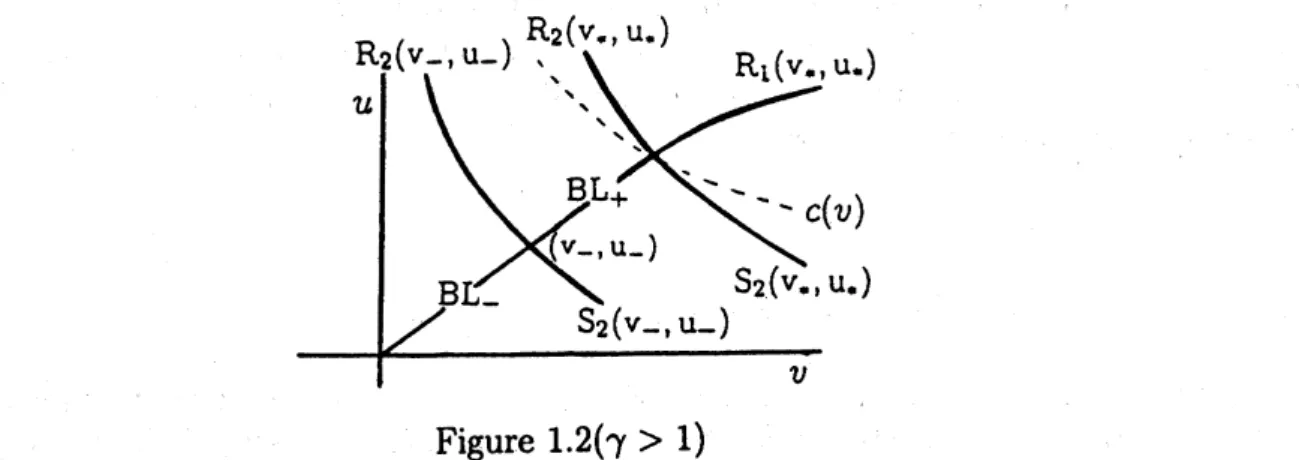
Hence, the large time behaviors to be expected devide the $(v, u)$-space as the

following figure, Figure 1.2.

Figure

1.2.

$>1$)

Here,

$BL_{+}(v_{-}, u_{-})=\{(v, u)\in BL(v_{-}, u_{-});v_{-}<v\leq v_{*}\}$

$BL_{-}(v_{-}, u_{-})=\{(v, u)\in BL(v_{-}, u_{-});0<v<v_{-\}}$ $R_{1}(v_{*}, u_{*})=$

{

$(v,$$u);u=u_{*}- \int_{v_{*}}^{v}$Xi_$(s)ds$, _{$v>v_{*}$}

}

$R_{2}(v_{-}, u_{-})= \{(v, u);u=\mathrm{v}\mathrm{z}_{-}-\int_{v-}^{v}\lambda_{2}(s)ds, v<v_{*}\}$

$R_{2}(v*’ u*)=$

{

$(v,$$u);u=u_{*}- \int_{v_{*}}^{v}$X2(s)ds, _{$v<v_{*}$}

}

$S_{2}(v_{-}, u_{-})=\{(v, u);u=\mathrm{t}\mathrm{z}_{-}-s_{2}(v-v_{-}), v>v_{-}\}$ $S_{2}(v_{*}, u_{*})=\{(v, u);u=u_{*}-s_{*}(v-v_{*}), v>v_{*}\}$,

(I) If $(v+’ u_{+})\in BL_{+}(v_{-}, u-)$, then the $\mathrm{B}\mathrm{L}$-solution

is stable.

(II) If $(v_{+}, u_{+})\in BL_{-}(v_{-}, u_{-})$ , then the $\mathrm{B}\mathrm{L}$-solution is stable provided that

$|(v_{+}-v_{-}, u_{+}-u_{-})|$ is small. That is, the $\mathrm{B}\mathrm{L}$-solution

is

necessary

to be weak.

(III) If $(v_{+}, u_{+})\in BL_{+}R_{2}(v_{-}, u-)$, then there exists $(\mathrm{v},\mathrm{u})\overline{u})\in BL_{+}(v_{-}, u_{-})$

such that $(v_{+}, u_{+})\in R_{2}(\overline{v},\overline{u})$, and the superposition of the $\mathrm{B}\mathrm{L}$-solution connect-$\mathrm{i}\mathrm{n}\mathrm{g}$ $(v_{-}, u_{-})$ with $(\overline{v},\overline{u})$ and the 2-rarefaction

wave

connecting

$(\overline{v},\overline{u})$ with _{$(v_{+}, u_{+})$}

is stableprovided that $|(v_{+}-\overline{v}, u_{+}-\overline{u})|$ is small, where

$BL_{+}R_{2}(v_{-}, u_{-})=$

{

$(v,$$u);u>-s_{-}v$, $u>u_{-}- \int_{v-}^{v}\lambda_{2}(s)ds$, $u \leq u_{*}-\int_{v}^{v}$

.X2

$(s)ds$

}.

That is, the rarefaction

wave

is weak, but the $\mathrm{B}\mathrm{L}$-solution is not

necessarily weak.

(IV) If $(v+’ u_{+})\in BL_{-}R_{2}(v_{-}, u-)$, then the superposition of the $\mathrm{B}\mathrm{L}$-solution and

the 2-rarefaction wave is stable provided that $|(v_{+}-v_{-}, u_{+}-u_{-})|$ is small, where

$BL_{-}R_{2}(v_{-}, u_{-})=$

{

(v, u);u $>-\mathrm{s}_{-}\mathrm{v}$, u $<u_{-}- \int_{v-}^{v}$X2$(s)ds$

}.

In this case, both the $\mathrm{B}\mathrm{L}$-solution and the rarefaction

wave are weak.

(V) If $(v_{*}, u_{*})\in BL_{+}(v_{-}, u-)$, $(v_{+}, u_{+})\in R_{1}R_{2}(v_{*}, u_{*})$ and _{$|(v_{+}-v_{*},$ $u_{+}-$}

$u_{*})|$ is small, then the superposition of the $\mathrm{B}\mathrm{L}$-solution, 1-rarefaction

wave

and

2-rarefaction

wave

is stable. Here,

$R_{1}R_{2}(v_{*}, u_{*})=$

{

(v,u);u $>u_{*}- \int_{v}^{v}$

.

Xi(s)ds, i $=1,$

2}.

Similar to (III), the $\mathrm{B}\mathrm{L}$-solution is not necessarily weak.

In the proofs of the above assertions, the sign of $U_{\xi}=V_{t}$ is important, similar

to those of the Cauchy problem. So, to show (/) and (II) are essential. The case

(III), $(\mathrm{I}/^{\ovalbox{\tt\small REJECT}})$ are the applications to (/), and (IV) is to (//). In the next section we

mainly state the stability thorems of the boundary layer solutions.

The other cases are still open. For example, when

$(v_{+}, u_{+})\in BL_{-}S_{2}(v_{-}, u_{-})=\{(v, u);u<-s_{-}v, u<u_{-}-s_{2}(v-v_{-})\}$,

theasmptoticstateis conjectured to be $(V, U)(x-s_{-}t)+(V_{2}^{S}, U_{2}^{S})(x-s_{2}t+\alpha)-(\overline{v},\overline{u})$

together with asuitable shift $\alpha$, where $(\overline{v},\overline{u})\in BL_{-}(v_{-}, u_{-})$ such that $(v_{+}, u_{+})\in$ $\mathrm{s}2\{\mathrm{v}\overline{u}$), and $(V, U)$ is the $\mathrm{B}\mathrm{L}$-solution connecting $(v_{-}, u_{-})$ with $(\overline{v},\overline{u})$ and $(V_{2}^{S}, U_{2}^{S})$

is 2-viscous shock

wave

connecting $(\overline{v},\overline{u})$ with $(v_{+}, u_{+})$. Even though the shift $\alpha$ is

conjectured by the

same

way

as

in Matsumura and Mei [3], this

case

is not solved

yet.

2Stability of the boundary layer

solution

2.1

The

case

$(v_{+}, u_{+})\in BL_{+}(v_{-}, u_{-})$

Assume that

$(\mathrm{V}, u_{-})\in\Omega_{sub}$ and $(v_{+}, u_{+})\in BL+(v_{-}, u_{-})$, (2.1)

then aboundarylayersolution $(V, U)(\xi)$, $\xi=x-s_{-}t\geq 0$, $s_{-}=-u_{-}/v_{-}$ connecting

$(v_{-}, u_{-})$ with $(v_{+}, u_{+})$ is uniquely determined in Lemma 1.1. Note that

$U_{\xi}=-s_{-}V_{\xi}>0$, (2.2)

which plays an important role in theapriori estimate. The perturbation $(\phi, \psi)(\xi, t)$

defined by

$(v, u)(x, t)=(V, U)(\xi)+(\phi, \psi)(\xi, t)$, (2.3)

satisfies

$\{$

$\phi_{t}-s_{-}\phi_{\xi}-\psi_{\xi}=0$, $\xi>0$, $t>0$

$\psi_{t}-s_{-}\psi_{\xi}+(p(V+\phi)-p(V))_{\xi}=\mu(\frac{U_{\xi}+\psi_{\xi}}{V+\phi}-\frac{U_{\xi}}{V})_{\xi}$

$(\phi, \psi)|_{\xi=0}=(0,0)$

$(\phi, \psi)|_{t=0}=(\phi_{0}, \psi_{0})(\xi):=(v_{0}-V, u_{0}-U)(\xi)$,

(2.4)

from (1.2) and (1.6).

To solve (2.4)

we

apply the $L^{2}$-energy method. The solution space is defined by

$X_{m,\Lambda f}(0, T)=\{(\phi, \psi)\in C([0, T];H_{0}^{1})|\phi_{x}\in L^{2}(0, T;L^{2})$, $\psi_{x}\in L^{2}(0, T;H^{1})$

with $\sup_{[0,T]}||(\phi, \psi)(t)||_{1}\leq M$, $\inf_{\mathrm{R}_{+}\cross[0,T]}(V+\phi)(\xi, t)\geq m\}$,

for positive constants $m$, $M$. Here, we denote $||f||_{k}=( \sum_{j=1}^{k}.||\partial_{x}^{j}f||^{2})^{1/2}$ and $||f||=$

$( \int_{0}^{\infty}|f(x)|^{2}dx)^{1/2}$. To obtain atime-globalsolution, we combine the time-local

exis-tence of the solution with the apriori estimates, which are given as follows

Proposition 2. 1(Local existence) Let ($o,$\ovalbox{\tt\small REJECT}\# 0$) be in $\mathrm{f}\mathrm{f}|3$(R.). $If|| 0$,

$\mathrm{e}_{0}||_{\mathrm{t}}\ovalbox{\tt\small REJECT}$

M and $\inf 4\mathrm{x}(0,T)(\mathrm{I}’+(4\rangle t)\ovalbox{\tt\small REJECT}_{\ovalbox{\tt\small REJECT}}m$, then there $e\ovalbox{\tt\small REJECT} ts$ $t_{0}\ovalbox{\tt\small REJECT}$ $t_{0}$(m,

A#)

$>0$ such that (24) has a unique solution ($, e) E $X_{4^{\ovalbox{\tt\small REJECT}\cdot,27\mathrm{H}}}(0, t_{0})$.

Proposition 2. 2(A priori estimates) Let $(\phi, \psi)$ be asolutionto (2.4) in $X_{\frac{1}{2}m,\epsilon}$

$(0, T)$. Then,

for

a suitably small$\epsilon$ $>0$, there exists a constant $C_{0}>0$

such that

$||( \phi, \psi)(t)||_{1}^{2}+\int_{0}^{t}(\psi_{\xi}(0, \tau)^{2}+||\sqrt{V_{\xi}}\phi(\tau)||^{2}+||\phi_{\xi}(\tau)||^{2}+||\psi_{\xi}(\tau)||_{1}^{2})d\tau\leq C_{0}||\phi_{0}$ _,$\psi_{0}||_{1}^{2}$.

Remark 2.1 If $\epsilon$ is suitably small, then

$\inf_{\mathrm{R}_{+}\mathrm{x}[0,T]}(V+\phi)(\xi, t)\geq m/4$ is

aut0-matically satisfies by the Sobolev inequality. Hence

we

denote $X_{m,\epsilon}(0, T)$ simply by

$X_{\frac{1}{2}\vee \mathrm{P}}(0, T)$.

The stability theorem is derived from these two Propositions in astandard way. Theorem 2. 1(Stability of$\mathrm{B}\mathrm{L}$ solution

$If||v_{0}-V$,$u_{0}-U||_{1}$ is suitably small

togetherwith the compatibility condition$(v_{0}-V, u_{0}-U)(0)=(0,0)$_, then there eists

a unique solution $(v, u)$ to (1.2), which satisfy $(v-V, u-U)\in C([0, \infty);H_{0}^{1})$ and

$\sup_{\epsilon\geq 0}|(\phi, \psi)(\xi, t)|=\sup_{x\geq s_{-}t}|(v, u)(x, t)-(V, U)(x-s_{-}t)|arrow 0$ as $tarrow\infty$.

We first sketch the proof of the local existence theorem, Propositions 2.1.

By $(2.4)_{1}$, $\phi$ has the explicit form

$\phi(\xi, t)=\{$

$\int_{t+_{\epsilon_{-}}}^{t}[perp]\psi_{\xi}(\xi+s_{-}(t-\tau), \tau)d\tau$, $0\leq\xi\leq-s_{-}t$

$\phi_{0}(\xi+s_{-}t)+\int_{0}^{t}\psi_{\xi}(\xi+s_{-}(t-\tau), \tau)d\tau$, _{$\xi\geq-s_{-}t$}.

(2.5)

$\mathrm{E}\mathrm{q}.(2.4)_{2}$ is written

as an

initial-boundary value problem for the linear parabolic equatioin of$\psi$:

$\{$

$\psi_{t}-\mu(\frac{\psi_{\xi}}{V+\phi})_{\xi}=g:=g(\psi_{\xi}, \phi, \phi_{\xi})$

$\psi(0, t)=0$

$\psi(\xi, 0)=\psi_{0}(\xi)$,

(2.6)

where

$g( \psi_{\xi}, \phi, \phi_{\xi})=s_{-}\psi_{\xi}-(p(V+\phi)-p(V))_{\xi}+\mu(\frac{U_{\xi}}{V+\phi}-\frac{U_{\xi}}{V})_{\xi}$ .

To

use

the iteration method,

we

approximate $(\phi_{0}, \psi_{0})\in H_{0}^{1}$ by $(\phi_{0k}, \psi_{0k})\in$ $H^{2}\cap H_{0}^{1}$ such that

(0,$\psi_{0k})arrow(\phi_{0}, \psi_{0})$ strongly in $H^{1}$

as $karrow\infty$. We may

assume

$||\phi_{0k}$,$\psi_{0k}||_{1}\leq\frac{3}{2}M$, $\inf_{\mathrm{R}_{+}}(V+\phi_{0k})\geq\frac{2}{3}m$

for any $k\geq 1$. Define the sequence $\{(\phi^{(n)}, \psi^{(n)})\}:=\{(\phi_{k}^{(n)}., \psi_{k}^{(n)}.)\}$for each $k$ so that

$(\phi^{(0)}, \psi^{(0)})(\xi, t)=(\phi_{0k}, \psi_{0k})(\xi)$ ,

and, for agiven $(\phi^{(n-1)}, \psi^{(n-1)})(\xi, t)$, $\psi^{(n)}$ is asolution to

$\{$

$\psi_{t}^{(n)}-\mu(\frac{\psi_{\xi}^{(n)}}{V+\phi^{(n-1)}})_{\xi}=g^{(n-1)}:=g(\psi(n-1)_{\xi}, \phi^{(n-1)}, \phi_{\xi}^{(n-1)})$

$\psi^{(n)}(0, t)=0$ $\psi^{(n)}(\xi, 0)=\psi_{0k}(\xi)$, $(2.6)’$ and $\phi^{(n)}(\xi, t)=$ .

$\int_{t\dagger_{s_{-}}^{\Delta_{-}^{\zeta}}}^{t}\psi_{\xi}^{(n)}(\xi+s_{-}(t-\tau), \tau)d\tau$, $0\leq\xi\leq-s_{-}t$

(2.5)’

$\backslash \phi_{0k}(\xi+s_{-}t)+\int_{0}^{t}\psi_{\xi}^{(n)}(\xi+s_{-}(t-\tau), \tau)d\tau$, $\xi\geq-s_{-}t$.

From the linear theory, if $g\in C^{0}([0, T];L^{2})$, $\psi_{0}\in H^{2}\cap H_{0}^{1}$, then there exists a

unique solution $\psi$ to (2.6) satisfying

$\psi$ $\in C([0, T];H^{2}\cap H_{0}^{1})\cap C^{1}([0, T];L^{2})\cap L^{2}(0, T;H^{3})$. Using this, if $(\phi^{(n-1)}, \psi^{(n-1)})\in X_{\frac{1}{2}m,2M}$ , then we have

$||( \phi^{(7l)}, \psi^{(7\iota)})(t)||^{2}\leq((\frac{3}{2}M)^{2}+C(m, M)t_{0})\exp(C_{/}(m, M)t_{0})$ _(2.7) $\leq(2M)^{2}$ if $0<t_{0}:=t_{0}(n\iota, M)<<1$

and also

$\int_{0}^{t_{\mathrm{O}}}||\psi_{\xi}^{(n)}(\tau)||_{1}^{2}d\tau\leq C(m, M)M^{2}$ .

Hence, direct estimates on (2.5)’ give

$|| \int_{t+_{\overline{s}_{-}}^{e}}^{t}=\psi_{\xi}^{(n)}(\xi+s_{-}(t-\tau), \tau)d\tau||_{1}\leq C\sqrt{t_{0}}M$

and

$|| \int_{0}^{t}\psi_{\xi}^{(n)}(\xi+s_{-}(t-\tau), \tau)d\tau||_{1}\leq C\sqrt{t_{0}}M$.

Hence, for asuitable small $t_{0}$

we

have

$\sup_{0\leq t\leq t_{\mathrm{O}}}||\phi^{(n)}(t)||_{1}\leq 2M$ and $\inf_{\mathrm{R}_{+}\mathrm{x}[0,t_{\mathrm{O}}]}(V+\phi)(\xi, t)\geq\frac{1}{2}m$. (2.8)

By (2.7)-(2.8), $(\phi^{(n)}, \psi^{(n)})\in X_{\frac{1}{2}m,2M}(0, t_{0})$. By a standard way,

$(\phi^{(n)}, \psi^{(n)})$

can

be shown to be the Cauchy sequence in $C([0, t_{0}];H^{1})$. Thus we have _asolution

$(\phi_{k}, \psi_{k})\in X_{\frac{1}{2}m,2\mathrm{A}\mathrm{f}}(0, t_{0})$ to(2.5) and (2.6) by

$\lim_{narrow\infty}(\phi^{(n)}, \psi^{(n)})=\lim_{narrow\infty}(\phi_{k}^{(n)}, \psi_{k}^{(n)}.)$.

Here,

we

note that

$\phi_{k}\in C([0, t_{0}];H^{2}\cap H_{0}^{1})$ and

$\psi_{k}\in C([0, t_{0}];H^{2}\cap H_{0}^{1})\cap C^{1}$($[0$,to]; $L^{2}$)

$\cap L^{2}(0, t_{0};H^{3})$,

since $g((\psi_{k})_{\xi}, \phi_{k}, (\phi_{k})_{\xi})\in C([0, t_{0}];L^{2})$ and

$(\phi_{0k}, \psi_{0k}.)\in H^{2}\cap H_{0}^{1}$. Again,

show-ing that $(\phi_{k}, \psi_{k})$ is aCauchy sequence in

$C_{/}([0, t_{0}];H^{1})$ (taking $t_{0}$ smaller than the previous

_one

if necessary),

we

obtain the desired unique-local _solution $(\phi, \psi)\in$

$X_{\frac{1}{2}m,2M}(0, t_{0})$.

Next, we show the apriori estimate.

Let $($$,$\psi)$ be asolution in

$X_{\frac{1}{2}m,\epsilon}(0, T)=X_{\epsilon}(0, T)$. First, Multiply $(2.4)_{1}$ and

$(2.4)_{2}$ by $\psi$ and $-(p(V+\phi)-p(V))$,

respectively, and add these two equations to

have adivergence form

$\{\frac{1}{2}\psi^{2}+\Phi(v, V)\}_{t}$ $+ \{s_{-}\Phi(v, V)-\frac{s_{-}}{2}\psi^{2}+(p(v)-p(V))\phi-\mu(\frac{\psi_{\xi}^{2}}{v}-\frac{U_{\xi}}{V})\psi\}_{\xi}$ _(2.9) $+ \{\mu\frac{\psi_{\xi}^{2}}{v}-\mu s_{-}\frac{V_{\xi}\phi\psi_{\xi}}{vV}-s_{-}V_{\xi}(p(V+\phi)-p(V)-p’(V)\phi)\}=0$ , where $\Phi(v, V)=p(V)\phi-\int_{V}^{V+\phi}p(\eta)dr_{l}$. _(2.10)

Here and after

we

will often

use

the notation $(v, u)=(V+\phi, U+\phi)$_{, though the}

unknown functions are $\phi$ and $\psi$. Since$\mathrm{p}(\mathrm{V})>0$, put

$p(V+\phi)-p(V)-p’(V)\phi=f(v, V)\phi^{2}$_{, (2.11)}

then $f(v, V)\geq 0$_. Hence _{(2.2) is} effective, _{and the last three terms in (2.9) are}

regarded as the quadratic equation:

$Q:= \mu\frac{\psi_{\xi}}{v}-\mu s_{-}\frac{V_{\xi}\phi\psi_{\xi}}{vV}-s_{-}V_{\xi}f(v, V)\phi^{2}$

$=( \sqrt{\mu}\frac{\psi_{\xi}}{\sqrt{v}})^{2}-\frac{\sqrt{-\mu s_{-}V_{\xi}}}{V\sqrt{vf(v,V)}}\cdot\sqrt{\mu}\frac{\psi_{\xi}}{\sqrt{v}}\cdot\sqrt{-s_{-}V_{\xi}f(v,V)}\phi+(\sqrt{-s_{-}V_{\xi}f(v,V)}\phi)^{2}$.

The discriminant of $Q$ is $D= \frac{-\mu s_{-}V_{\xi}}{V^{2}vf(v,V)}-4=\frac{-h(V)}{Vvf(v,V)}-4$. (2.12) Since $v_{+}>v_{-}$, $-h(V)=s_{-}^{2}(V-v_{+})+p(V)-p(v_{+})<p(V)=V^{-\gamma}$. (2.13) Moreover, by putting $X=V/v$, $Vvf(v, V)= \frac{Vv(v^{-\gamma}-V^{-\gamma}+\gamma V^{-\gamma-1}(v-V))}{(v-V)^{2}}$ (2.14)

$=V^{-\gamma} \cdot\frac{X^{\gamma+1}-(\gamma+1)X+\gamma}{(X-1)^{2}}\geq\gamma V^{-\gamma}$,

because $X^{\gamma+1}-(\gamma+1)X+\gamma\geq\gamma(X-1)^{2}$ for $X\geq 0$. By (2.12)-(2.14),

$D \leq\frac{V^{-\gamma}}{\gamma V^{-\gamma}}-4=\frac{1}{\gamma}-4\leq 3$. (2.15)

Thus, integrating (2.9)

over

$(0, \infty)$ $\cross(0, t)$, we have the following basic estimate.

Lemma 2. 1(Basic estimate) Forthe solution $(\phi, \psi)\in X_{\epsilon}(0, T)$, it holds that

$\frac{1}{2}||\psi(t)||^{2}+\int_{0}^{\infty}\Phi(v, V)(\xi, t)d\xi$

$+C_{/}^{-1} \int_{0}^{t}\int_{0}^{\infty}\{\frac{\psi_{\xi}^{2}}{v}+|\frac{V_{\xi}\phi\psi_{\xi}}{vV}|+(p(V+\phi)-p(V)-p’(V)\phi)V_{\xi}\}d\xi d\tau$

$\leq\frac{1}{2}||\psi_{0}||^{2}+\int_{0}^{\infty}\Phi(v_{0}, V)(\xi)d\xi\leq C||\phi_{0}$,$\psi_{0}||^{2}$.

Next, following [7], change $\phi$ to $\tilde{v}:=v/V$. Since

$p(V+\phi)-p(V)-p’(V)\phi=V^{-\gamma}(\tilde{v}^{-\gamma}-1+\gamma(\tilde{v}-1))$ and $\Phi(v, V)=V^{-\gamma+1}\tilde{\Phi}(\tilde{v})$, where $\tilde{\Phi}(\tilde{v})=\{$ $\tilde{v}-1-\ln\tilde{v}$ $(\gamma=1)$ $\tilde{v}-1+\frac{1}{\gamma-1}(\tilde{v}^{-\gamma+1}-1)$ $(\gamma>1)$,

Lemma 2.1 is rewritten as follows

Lemma 2. 2It

_follows

that

$\frac{1}{2}||\psi(t)||^{2}+\int_{0}^{\infty}V^{-\gamma+1}\tilde{\Phi}(\tilde{v}(\xi, t))d\xi$

$+C^{-1} \int_{0}^{t}\int_{0}^{\infty}\{\frac{\psi_{\xi}^{2}}{v}+|\frac{V_{\xi}\phi\psi_{\xi}}{vV}|+\frac{V_{\xi}}{V^{\gamma}}(\tilde{v}^{-\gamma}-1+\gamma(\tilde{v}-1))\}d\xi d\tau$

$\leq C||\phi_{0}$,$\psi_{0}||^{2}$. Eq. $(2.4)_{2}$ is also written

as

$( \mu\frac{\tilde{v}_{\xi}}{\tilde{v}}-\psi)_{t}-s_{-}(\mu\frac{\tilde{v}_{\xi}}{\tilde{v}}-\psi)_{\xi}+\frac{\gamma\tilde{v}_{\xi}}{V^{\gamma}\tilde{v}^{\gamma+1}}+\frac{\gamma V_{\xi}}{V^{\gamma+1}}(\tilde{v}^{-\gamma}-1)=0$

. (2.16)

Multiplying (2.16) by $\tilde{v}_{\xi}/\tilde{v}$,

we

have adivergence form

$\{\frac{\mu}{2}(\frac{\tilde{v}_{\xi}}{\tilde{v}})^{2}-\psi(\frac{\tilde{v}_{\xi}}{\tilde{v}})\}_{t}$

$+ \{\psi\frac{v_{t}}{v}-\frac{\gamma h(V)}{s_{-}\mu V^{\gamma}}(\frac{\tilde{v}^{-\gamma}-1}{\gamma}+\ln\tilde{v})-\frac{\mu s_{-}}{2}(\frac{\tilde{v}_{\xi}}{\tilde{v}})^{2}\}_{\xi}+\frac{\gamma\tilde{v}_{\xi}^{2}}{V^{\gamma}\tilde{v}^{\gamma+2}}$

(2.17)

$= \frac{\psi_{\xi}^{2}}{v}+\frac{s_{-}\phi\psi_{\xi}V_{\xi}}{vV}-\frac{\gamma V_{\xi}}{s_{-}\mu}\frac{h’(V)V^{\gamma}-h(V)\gamma V^{\gamma-1}}{V^{2\gamma}}\{\frac{\tilde{v}^{-\gamma}-1}{\gamma}+\ln\tilde{v}\}$ .

By (2.2)

$|\mathrm{t}\mathrm{h}\mathrm{e}$ final term of $(2.14)| \leq C\frac{V_{\xi}}{V^{\gamma}}(\tilde{v}^{-\gamma}-1+\gamma(\tilde{v}-1))$

.

Hence, the right hand side of$(2.!4)$ is controllable _{by Lemma 2.2. Thus integrating}

(2.14)

over

$(0, \infty)$ $\cross(0, t)$ yields the following lemma.

Lemma 2. 3It holds that

$|| \frac{\tilde{v}_{\xi}}{\tilde{v}}(t)||^{2}+\int_{0}^{t}\int_{0}^{\infty}.\frac{\tilde{v}_{\xi}^{2}}{\tilde{v}^{\gamma+2}}d\xi d\tau$

(2.18)

$\leq C(||\phi_{0}||_{1}^{2}+||\psi_{0}||^{2})+C\int_{0}^{t}(\frac{\tilde{v}_{\xi}}{\tilde{v}})^{2}(0, \tau)d\tau$.

We note that the estimates until

now

have been obtained without smallness

condition. Hence we wish to control the final term of (2.18), $C \int_{0}^{t\overline{v}}(_{\overline{v}}^{4})^{2}(0, \tau)d\tau$,

without smallness condition, in asimilar fashion to $[6,7]$. But, we could not do it. However, we can control it provided that the initial data is small. Since

$( \frac{\tilde{v}_{\xi}}{\tilde{v}})^{2}(0, \tau)=\frac{1}{v_{-}^{2}}\phi_{\xi}^{2}(0, \tau)=\frac{1}{u_{-}^{2}}\psi_{\xi}^{2}(0, \tau)\leq C||\psi_{\xi}(\tau)||||\psi_{\xi\xi}(\tau)||$, (2.19)

it is necessary to estimate $I\ovalbox{\tt\small REJECT}\ovalbox{\tt\small REJECT}_{\ovalbox{\tt\small REJECT}}^{\ovalbox{\tt\small REJECT}_{\ovalbox{\tt\small REJECT}}}\ovalbox{\tt\small REJECT} l<)_{q_{t};}\ovalbox{\tt\small REJECT} r$) $|^{\ovalbox{\tt\small REJECT}}|^{2}dr$, which is controllable for small the initial

data.

We now

assume

that

$N(T):= \sup_{0\leq t\leq T}||(\phi, \psi)(t)||_{1}\leq\in$ $<<1$.

Multiplying $(2.4)_{2}\mathrm{b}\mathrm{y}-\psi_{\xi\xi}$,

we

have

$( \frac{1}{2}\psi_{\xi}^{2})_{t}+(-\psi_{t}\psi_{\xi}+\frac{s_{-}}{2}\psi_{\xi}^{2})_{\xi}+\mu\frac{\psi_{\xi\xi}^{2}}{v}$

$= \{-\mu\frac{\psi_{\xi}(V_{\xi}+\phi_{\xi})}{(V+\phi)^{2}}+\mu(\frac{U_{\xi}}{V+\phi}-\frac{U_{\xi}}{V})_{\xi}-(p(V+\phi)-p(V))_{\xi}\}(-\psi_{\xi\xi})$

and, after integrating the resultant equation

over

$(0, \infty)$ $\cross(0, t)$,

$|| \psi_{\xi}(t)||^{2}+\int_{0}^{t}(\psi_{\xi}(0, \tau)^{2}+||\psi_{\xi\xi}(\tau)||^{2})d\tau$

(2.20) $\leq C||\psi_{0\xi}||^{2}+C\int_{0}^{t}\int_{0}^{\infty}(\phi_{\xi}^{2}+V_{\xi}\phi^{2}+\psi_{\xi}^{2})d\xi d\tau$.

Here, we have estimated the amount $(\phi\xi\psi\xi)^{2}$ as

$\int_{0}^{t}\int_{0}^{\infty}(\phi_{\xi}\psi_{\xi})^{2}d\xi d\tau\leq\int_{0}^{t}||\psi_{\xi}||||\psi_{\xi\xi}||||\phi_{\xi}||^{2}d\tau$

$\leq lJ$ $\int_{0}^{t}||\psi_{\xi\xi}||^{2}d\tau+C_{\nu}N(T)^{2}\int_{0}^{t}||\phi_{\xi}(\tau)||^{2}d\tau$

for asmall constant $|J$ $>0$. By Lemma 2.1, (2.20) is reduced to

$|| \psi_{\xi}(t)||^{2}+\int_{0}^{t}(\psi_{\xi}(0, \tau)^{2}+||\psi_{\xi\xi}(\tau)||^{2})d\tau$

(2.21)

$\leq C(||\phi_{0}||^{2}+||\psi_{0}||_{1}^{2})+C\int_{0}^{t}||\phi_{\xi}(\tau)||^{2}d\tau$.

For asmall constant $\lambda>0$, (2.18)+(2.21) $\cdot\lambda$ together with (2.19) yield

$|| \frac{\tilde{v}_{\xi}}{\tilde{v}}(t)||^{2}+\lambda||\psi_{\xi}(t)||^{2}+\int_{0}^{t}(||\tilde{v}_{\xi}(\tau)||^{2}+\lambda\psi_{\xi}(0, \tau)^{2}+\lambda||\psi_{\xi\xi}(\tau)||^{2})d\tau$

$\leq C||\phi_{0}$,$\psi_{0}||_{1}^{2}+C\int_{0}^{t}((\frac{\tilde{v}_{\xi}}{\tilde{v}})^{2}(0, \tau)+\lambda||\phi_{\xi}(\tau)||^{2})d\tau$

$\leq C||\phi_{0}$,$\psi_{0}||^{2}+\int_{0}^{t}(_{\mathfrak{l}\prime}||\psi_{\xi\xi}(\tau)||^{2}+C_{\mathfrak{l}/}/||\psi_{\xi}(\tau)||^{2}+C\lambda||\phi_{\xi}(\tau)||^{2})d\tau$ .

$|| \tilde{v}_{\xi}(t)||^{2}=\int_{0}^{\infty}(\frac{\phi_{\xi}}{V}-\frac{V_{\xi}\phi}{V^{2}})^{2}d\xi$

$\geq\int_{0}^{\infty}(\frac{\phi_{\xi}^{2}}{2V^{2}}-\frac{(V_{\xi}\phi)^{2}}{V^{4}})d\xi\geq c_{0}||\phi_{\xi}(t)||^{2}-C||\phi(t)||^{2}$

and

$\int_{0}^{t}||\tilde{v}_{\xi}(\tau)||^{2}d\tau\geq \mathrm{q}_{1}\int_{0}^{t}||\phi_{\xi}(\tau)||^{2}d\tau-C\int_{0}^{t}\int_{0}^{\infty}V_{\xi}\phi^{2}d\xi d\tau$ ,

we fix Asuch that $C\lambda\leq \mathrm{q}_{1}/2$ and $l/$ such that $|/\leq\lambda/2$. Then, the following lemma

holds.

Lemma 2.

_4If

$N(T)= \sup_{0\leq t\leq T}||(\phi, \psi)(t)||_{1}$ _is suitably small, then

$||( \phi_{\xi}, \psi_{\xi})(t)||^{2}+\int_{0}^{t}(\psi_{\xi}(0, \tau)^{2}+||(\phi_{\xi}, \psi_{\xi\xi})(\tau)||^{2})d_{\mathcal{T}}\leq C||\phi_{0}$,$\psi_{0}||_{1}^{2}$.

Combining Lemmas 2.1-2.4 completes the proofof Proposition 2.2.

We briefly mention thecase $(v_{+}, u_{+})\in BL_{+}R_{2}(v_{-}, \mathrm{u}_{-})$, $R_{1}(v_{*}, u_{*})$ or$R_{1}R_{2}(v_{*}, u_{*})$.

For example, for $(v_{+}, u_{+})\in BL_{+}R_{2}(v_{-}, u-)$, there is aunique $(\mathrm{v},\mathrm{u})\overline{u})\in BL_{+}$ such

that $(v_{+}, u_{+})\in R_{2}(\overline{v},\overline{u})$, and there exist

a

$\mathrm{B}\mathrm{L}$ solution

$(V_{0}, U_{0})(x-s_{-}t)$ connecting

$(v_{-}, u_{-})$ with $(\overline{v},\overline{u})$ and a2-rarefaction

wave

$(v_{2}^{R}, u_{2}^{R})(x/t)$ connecting $(\overline{v},\overline{u})$ with

$(v_{+}, u_{+})$. The behavior of solution _{$(v, u)$} to (1.2) is expected to be

$(v, u)(x, t)\sim(\mathrm{V}\mathrm{o}’-\mathrm{S}-\mathrm{t})+v_{2}^{R}(x/t)-\overline{v},$$U_{0}(x-\mathrm{S}-\mathrm{t})+u_{2}^{R}(x/t)-\overline{u})$ (2.22)

as

$tarrow\infty$. To show (2.22)

we

first construct asmoothapproximate rarefaction wave

$(V_{2}, U_{2})(x, t)$ satisfying

$\{$

$V_{2t}-U_{2x}=0$

$U_{2t}+p(V_{2})_{x}=0$

with $U_{2x}=V_{2t}>0$ and $\lim_{tarrow\infty}\sup|(V_{2}, U_{2})(x, t)-(v_{2}^{R}, u_{2}^{R})(x/t)|=0(\mathrm{S}\mathrm{e}\mathrm{e}[5,6,7])$.

Then, the perturbation $(\phi, \psi)(\xi, t)=(v-(V_{0}+V_{1}-\mathrm{u}_{-}), u-(U_{0}+U_{1}-\mathrm{u}))=$:

$(v-V, u-U)$ satisfies

$\{$

$\phi_{t}-s_{-}\phi_{\zeta}-\psi_{\xi}=0$

$\psi_{t}-s_{-}\psi_{\xi}+(p(V+\phi)-p(V))_{\xi}=\mu(\frac{U_{0\xi}+\psi_{\xi}}{V_{0}+\phi}-\frac{U_{0\xi}}{V_{0}})_{\xi}$

$-(p(V)-p(V_{0})-p(V_{1})+p(\overline{v}))_{\xi}$

$(\phi, \psi)|_{\xi=0}=(V_{1}-\overline{v}, U_{1}-\overline{u})|_{\xi=0}=:(\mathrm{v}, b_{U})(t)$

$(\phi, \psi)|_{t=0}=(v_{0}-V|_{t=0}, u_{0}-U|_{t=0})=:(\phi_{0},\psi_{0})(\xi)$.

(2.23)

Since the last term of $(2.23)_{2}$ and the boundary value $(b_{V}, b_{U})(t)$ are small as

$tarrow\infty$ if $|(v_{+}-\overline{v}, u_{+}-\overline{u})|<<1$, we can treat (2.23) as essentially same as (2.4).

In particular, since $U_{\xi}=U_{0\xi}+U_{1\xi}>0$, the basic estimate similar to Lemma 2.1 is

obtained, and hence the stability theorem for $(V, U)=(V_{0}+V_{1}-\overline{v}, U_{0}+U_{1}-\overline{u})$

holds provided that $|(v_{+}-\overline{v}, u_{+}-\overline{u})|<<1$. Weomit the details

2.2

The

case

$(v_{+}, u_{+})\in BL_{-}(v_{-}, u_{-})$

In this subsection we assume that

$(v_{-}, u_{-})\in\Omega_{sub}$ and $(v_{+}, u_{+})\in BL_{-}(v_{-}, u_{-})$.

The situations

are

all

same as

the

case

$(v_{+}, u_{+})\in BL_{+}(v_{-}, u_{-})$ except for $\mu V_{\xi}=$ $\frac{V}{s-}l\iota(V)<0$. Hence, the perturbation $(\phi, \psi)$ satisfies (2.4), but the proofof Lemma

2.1 is not available. In this case, we have, from (2.9),

$\frac{d}{dt}\int_{0}^{\infty}(\frac{1}{2}\psi^{2}+\Phi(v, V))d\xi+\int_{0}^{\infty}\mu\frac{\psi_{\xi}^{2}}{v}d\xi$

$\leq C\int_{0}^{\infty}|V_{\xi}|\phi^{2}d\xi+lJ$$\int_{0}^{\infty}\psi_{\xi}^{2}d\xi+C_{\nu}\int_{0}^{\infty}|V_{\xi}|^{2}\phi^{2}d\xi$

for asmall constant $\mathfrak{l}J>0$. If$\delta=|(v_{+}-v_{-}, u_{+}-u_{-})|<<1$ and $||(\phi, \psi)(t)||_{1}\leq\in$$<<1$, then

$||( \phi, \psi)(t)||^{2}+\int_{0}^{t}||\psi_{\xi}(\tau)||^{2}d\tau\leq C||\phi_{0}$,$\psi_{0}||^{2}+C\int_{0}^{t}\int_{0}^{\infty}|V_{\xi}|\phi(\xi, \tau)^{2}d\xi d\tau$. (2.24)

The estimate of the last term is akey point. Applying the idea by Kawashima and

Nikkuni [1], we have

$\phi(\xi, t)=\phi(0, t)+\int_{0}^{\xi}\phi_{\xi}(\eta, t)d\eta\leq\xi^{1/2}||\phi_{\xi}(t)||$ ,

and

$C \int_{0}^{t}\int_{0}^{\infty}|V_{\xi}|\phi(\xi, \tau)^{2}d\xi d\tau\leq C\int_{0}^{t}||\phi_{\xi}(\tau)||^{2}\int_{0}^{\infty}\xi(-V_{\xi}(\xi))d\xi d\tau\leq C\delta\int_{0}^{t}||\phi_{\xi}(\tau)||^{2}d\tau$.

Thus we have

$||( \phi, \psi)(t)||^{2}+\int_{0}^{t}||\psi_{\xi}(\tau)||^{2}d\tau\leq C(||\phi_{0}, \psi_{0}||^{2}+\delta\int_{0}^{t}||\phi_{\xi}(\tau)||^{2}d\tau)$. (2.25)

Moreover we seek for the estimates of higher order derivatives.

Similar to the proof of Lemma 2.3, we can show

$|| \phi_{\xi}(t)||^{2}+\int_{0}^{t}||\phi_{\xi}(\tau)||^{2}d\tau\leq C(||\phi_{0}, \psi_{0}||_{1}^{2}+\int_{0}^{t}\phi_{\xi}(0, t)^{2}d\tau+\int_{0}^{t}\int_{0}^{\infty}|V_{\xi}|\phi^{2}d\xi d\tau)$ . (2.26)

Since

$C \int_{0}^{t}\phi_{\xi}(0, \tau)^{2}d\tau=\frac{c_{/}}{s_{-}^{2}}J_{0}^{t}.\psi_{\xi}(0, \tau)^{2}\leq \mathfrak{l}J\int_{0}^{t}||\psi_{\xi\xi}(\tau)||^{2}d\tau+C_{\nu}\int_{0}^{t}||\psi_{\xi}(\tau)||^{2}d\tau$,

(2.26) yields

$|| \phi_{\xi}(t)||^{2}+\int_{0}^{t}||\phi_{\xi}(\tau)||^{2}d\tau$

(2.27)

$\leq(||\phi_{0}, \psi_{0}||_{1}^{2})+\int_{0}^{t}\{|/||\psi_{\xi\xi}(\tau)||^{2}+C\delta||\phi_{\xi}(\tau)||^{2}+C_{/}’/||\psi_{\xi}(\tau)||^{2}\}d\tau$.

Further

we

have, by multiplying $(2.4)_{1}\mathrm{b}\mathrm{y}-\psi_{\xi\xi}$,

$|| \psi_{\xi}(t)||^{2}+\int_{0}^{t}(\psi_{\xi}(0, \tau)^{2}+||\psi_{\xi\xi}(\tau)||^{2})d\tau$

$\leq C||\phi_{0}$,$\psi_{0}||_{1}^{2}+C\int_{0}^{t}(||\phi_{\xi}(\tau)||^{2}+||\psi_{\xi}(\tau)||^{2})d\tau$.

(2.28)

Add (2.27) to A-(2.28) _{for afixed number} $\lambda>0$ such

as

_{$1-C\lambda\geq 1/2$ and}

$\nu=\lambda/2$, then

$||( \phi_{\xi}, \psi_{\xi})(t)||^{2}+\int_{0}^{t}(\psi_{\xi}(0, \tau)^{2}+||\phi_{\xi}(\tau)||^{2}+||\psi_{\xi\xi}(\tau)||^{2})d\tau$

$\leq C(||\phi_{0}, \psi_{0}||_{1}^{2}+\int_{0}^{t}||\psi_{\xi}(\tau)||^{2}d\tau)$.

(2.29)

Again, add (2.29)$\cdot\lambda(\lambda>0)$ to (2.25), then $||(\phi, \psi)(t)||^{2}+\lambda||(\phi_{\xi}, \psi_{\xi})(t)||^{2}$

$+ \int_{0}^{t}\{(1-C\lambda)||\psi_{\xi}(\tau)||^{2}+\lambda(\psi_{\xi}(0, \tau)^{2}+||\phi_{\xi}(\tau)||^{2}+||\psi_{\xi\xi}(\tau)||^{2}\}d\tau$

$\leq C||\phi_{0}$,$\psi_{0}||_{1}^{2}+C\delta\int_{0}^{t}||\phi_{\xi}(\tau)||^{2}d\tau$

.

Taking Aas $1-C\lambda\geq 1/2$ and restrict $\delta$

as

$\lambda-C\delta\geq\lambda/2$,

we

obtain the desired a

priori estimate.

Thus

we

reach thefollowing theorem.

Theorem 2.

_2If

$|v_{+}-v_{-}$,_{$u_{+}-u_{-}|+||v_{0}-V$},$u_{0}-U||_{1}$ _is suitably small with

the compatibility condition $(v_{0}-V, u_{0}-U)(0)=(0,0)$_{, then there eists a unique}

solution $(v, u)$ to (1.2), which

satisfies

$(v-V, u-U)\in C([0, \infty);H_{0}^{1})$ and $\sup_{x\geq s_{-}t}|(v, u)(x, t)-(V, U)(x-s_{-}t)|arrow \mathrm{O}$

as

$tarrow\infty$.

References

[1] S. Kawashima and Y. Nikkuni, Stability of stationary solutions to the half-space problem for the discrete Boltzmann equation with multiple collisions, Kyushu

J. Math., to appear.

[2] A. Matsumura, Inflow and outflow problems in the half space for

aone-dimensional isentropic model system ofcompressible viscous gas, Proceedings

ofIMS Conference onDifferential Equationsfrom Mechnics, Hong Kong, 1999.,

to appear.

[3] A. Matsumura and M. Mei, Convergence to traveling fronts of solutions ofthe psystem with viscosity in the presence of aboundary, Arch. Rat. Mech. Anal.

146(1999), 1-22

[4] A. Matsumura and K. Nishihara, On the stability oftraveling wavesolutions of

aone-dimensional model system for compressible viscous gas, Japan J. Appl.

Math. $2(1985)$, 17-25.

[5] –, Asymptotics toward the rarefaction waves of the solutions of

aone-dimensional model system for compressible viscous gas, Jpn. J. Appl. Math.

$3(1986)$, 1-13.

[6] –, Global stability ofthe rarefaction

wave

of

aone-dimensional

model system

for compressible viscous gas, Commun. Math. Phys. 144(1992),

325-335.

[7] –, Global asymptotics toward the rarefaction

wave

for solutions of viscous

psystem with boundary effect, Q. Appl. Math. 58(2000),

69-83.

[8] –, Large-time behaviors of solutions to

an

inflow problem in the half space

for

aone-dimensional

system of compressible viscous

gas,

preprint