Enumerating Colored and Rooted Outerplanar Graphs

全文

(1)Vol.2010-AL-129 No.5 2010/3/5 IPSJ SIG Technical Report. representation, and then define a parent-child relationship among all canonical representations such that the difference between parent-child embeddings is small, which is implicitly represented as the family tree each of whose nodes corresponds to the canonical representation of a graph. This indicates that all canonical representations can be enumerated one by one according to the depth-first traversal of the family tree. In this paper, we consider the problem of enumerating all colored and rooted outerplanar graphs with at most given n (≥ 1) vertices without repetition. To our best knowledge, few papers have been worked for this problem. The reasons are twofolds: 1) few researchers notice potential applications of the exhaustive list of outerplanar graphs, and 2) it is difficult to design efficient algorithms because free symmetry at cut-vertices and reflectional symmetry at rooted blocks lead to isomorphic duplications. We design an efficient algorithm that can enumerate all required outerplanar graphs in O(1) per each and in O(n) space. The algorithm proposed in this paper may have potential applications in various areas such as chemoinformatics, medicine and computer science.. Enumerating Colored and Rooted Outerplanar Graphs Jiexun Wang†1 and Hiroshi Nagamochi†1 An outerplanar graph is a graph that admits a planar embedding such that all vertices appear on the boundary of its outer face. Given a positive integer n and a color set C with K ≥ 1 colors, we consider the problem of enumerating all colored and rooted outerplanar graphs with at most n vertices without repetition. We design an efficient algorithm that can generate all required graphs in O(1) time per each and in O(n) space.. 1. Introduction The problem of enumerating (or listing) graphs of specific classes without repetition is one of fundamental and important problems in computer science. Various types of graphs has been studied such as trees7)–10) and series-parallel graphs5) . The graphical enumeration has been served as a very useful tool for solving problems in various field such as chemistry2),6) and biology3) . The goal of graphical enumeration problems is to efficiently enumerate graphs in classes without duplications in terms of running time and space. The running time (resp., space) of an enumeration algorithm is the time (resp., computer memory) required to compute the total amount of changes in the data structures, but not the time (resp., memory) required to print out all graphs. Particularly, many researchers are interested in the computation time per each graph, i.e., the delay between two successive outputs7),9) . Note that graphical symmetry leads to isomorphic duplications which prevent from designing efficient enumeration algorithms. In literature, there are various approaches developed for graphical enumeration problems1),4),5) . The common idea behind most of efficient algorithms is to first define a unique embedding for each graph to be enumerated as its canonical. 2. Preliminaries Throughout this paper, a graph stands for a simple connected undirected graph. The set of vertices and the set of edges of a graph H are denoted by V (H) and E(H), respectively. A graph is called planar if its vertices and edges can be drawn as points and curves on the plane so that no two curves intersect except for their endpoints. An outerplanar graph is a planar graph that admits a plane graph such that all vertices appear on the boundary of its outer face. A rooted graph is a graph with an arbitrary vertex designated as the root. For each block B of a graph rooted at a vertex r, the root r(B) of B is defined to be the unique vertex v ∈ V (B) closest to r. Let V ′ (B) denote V (B) − {r(B)}. A block B is called the parent-block of all other vertices in V ′ (B). A block B with r(B) = v is a child-block of v. The depth d(B) of a rooted block B is defined by the number of blocks which edge sets intersect with a simple path from a vertex in V ′ (B) to the root r. Let Br be an imaginary block which is the parent-block of rG , and define depth d(Br ) = 0. For two blocks B and B ′ with r(B ′ ) ∈ V ′ (B), we. †1 Department of Applied Mathematics and Physics, Kyoto University. 1. c 2010 Information Processing Society of Japan.

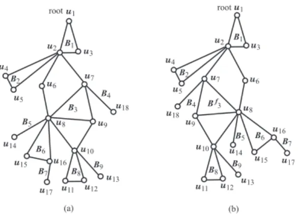
(2) Vol.2010-AL-129 No.5 2010/3/5 IPSJ SIG Technical Report root u1. root u1. 3. Rooted Outerplanar Graphs u2. u2 B 1. u3. B2. u7. u6. u18. B3. u14 u15. u8. u9. B4 u18. u6. B f3. u8. u9. u16 B7. u10. u10 B8. u17 u11 (a). Fig. 1. u7. B5 B6. Let G be a colored and rooted outerplanar embedding, and let rG denote the root of G. We define the depth d(rG ) = 0 for the root rG , and depth of other vertices in G recursively based on the following decomposition of blocks. 3.1 Structure of rooted blocks We decompose a rooted block B into three parts: “core,” “left wings” and “right wings,” where the core is a subgraph which is reflectionally symmetric in the block B (except for an assignment of colors to the vertices in the core), left (resp., right) wings can be treated as rooted outerplanar embeddings on the left (resp., right) side of B. Specifically, for a block B in G, the vertices in V ′ (B) adjacent to r(B) are called the head-vertices of B, and the edges in B incident to r(B) are called the head-edges of B. Let Vhead (B) denote the set of all head-vertices in B, and let h = |Vhead (B)|. We denote the head-vertices in Vhead (B) by x1 , x2 , . . . , x(h−1)/2 , z, y(h−1)/2, . . . , y2 , y1 (if h is odd) x1 , x2 , . . . , xh/2 , yh/2 , yh/2−1 , . . . , y2 , y1 (if h is even) from left to right, where x1 is the leftmost vertex in V (B) adjacent to r(B). See Fig. 2. Define depth of the above head-vertices to be d(xi ) = d(yi ) = d(r(B)) + i, d(z) = d(r(B)) + (h + 1)/2. We define “axial-faces,” “axial-vertex” and “bottom” of block B as follows. Let h be odd. We call vertex z the bottom vertex of B and denote it by bv(B). If h = 1, then no axial-face is defined for B. If h ≥ 3, then an inner face of B containing edge (r(B), z) is called an axial-face of B. Note that B has exactly two such faces. Let h be even. The inner face f1 of B containing both edges (r(B), xh/2 ) and (r(B), yh/2 ) is called the first axial-face of B. If f1 consists of an odd number of edges, then f1 has a unique edge e1 farthest from r(B), and the other inner face containing e1 (if any) is defined to be the second axial-face f2 . For each axial-face fi , i ≥ 2, if fi consists of an even number of edges, then fi has a unique edge ei farthest from r(B), and the other inner face containing ei (if any) is defined to be the (i + 1)st axial-face fi+1 . Given any block B, the non-head-vertices in all axial-faces are called the axial-. u5. B4. u5 B5. u3. u4. u4 B2. B1. B9. B8. u13 u12. u11. u14 B9 u12. B6 u15. u16 B7 u17. u13. (b). (a) An embedding G of a rooted outerplanar graph; (b) The embedding G′ obtained by flipping block B3 of G.. say that B is the parent-block of B ′ and that B ′ is a child-block of B. Similarly, we define the ancestor-blocks and descendant-blocks. Let C be a set of colors. A colored graph is a graph in which each vertex v is assigned with a color c(v) ∈ C (different vertices can receive the same color). Two colored and rooted graphs H1 and H2 are rooted-isomorphic if and only if their vertex sets admit a bijection by which the root, the color classes, and the incidence-relation between vertices and edges in H1 correspond to those in H2 . Note that two distinct embeddings of a colored and rooted graph are rootedisomorphic. A colored and rooted outerplanar graph H can have several different embeddings in the plane, where each embedding is determined by choosing one of the two ways of embeddings of each block and choosing one of the orderings of childblocks of each cut-vertex. We let G(B) denote the embedding of that consists of embeddings of B and all descendant-blocks of B. For an embedding G, let Gf denote the flipped embedding of G that is obtained by reversing the embedding G on the plane. For example, Fig. 1(a) shows an embedding G of a rooted outerplanar graph, and Fig. 1(b) shows the embedding G′ obtained by flipping block B3 in G.. 2. c 2010 Information Processing Society of Japan.

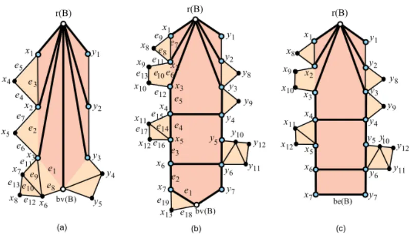
(3) Vol.2010-AL-129 No.5 2010/3/5 IPSJ SIG Technical Report. Fig. 2. B ′ if any. We define a unique numbering for the wing-vertices in B(x, x′ ) as the reverse order of the following vertex eliminations: recursively eliminating the wing-vertex of degree 2 visited last when traversing the boundary of B(x, x′ ) from x to x′ until no wing-vertices in B(x, x′ ) remains (Fig. 2). Besides, we define a unique numbering π for all wing-vertices in B(xi , xi+1 ) for i = 1, 2, . . . , p − 1 (and in B(xp , bv(B)) if bv(B) exists). The depth of the jth wing-vertex w in π is defined to be d(w) = d(r(B)) + p + j (see Fig. 2). The sequence of core-vertices x1 , x2 , . . . , xp and wing-vertices in the order π is called the left side of B. We define the right side of B in the same way (note that bv(B) is not contained in the left or right side of B). Let V L (B) and V R (B) denote the sets of vertices in the left and right sides of B, respectively. A vertex u ∈ V L (B) (resp., V R (B)) is called a left (resp., right) vertex of B. Also denote L R L R V L (B) ∩ Vcore (B) by Vcore (B). Similarly for Vcore (B), Vhead (B) and Vhead (B), L R L R Vaxis (B), Vaxis (B), Vwing (B) and Vwing (B). For a vertex u in the left side of B, let PL (u; B) denote the boundary of the left side of B from u to the bottom of B (excluding the bottom edge), and EL (u; B) denote the sequence of edges in the path PL (u; B). We define PR (u; B) and ER (u; B) for the right side symmetrically with PL (u; B) and EL (u; B). ˜ Let E(B) denote the set of all edges (v, v ′ ) with v, v ∈ V L (B) ∪ {bv(B)} or v, v ∈ V R (B) ∪ {bv(B)}, where we include edge (v, v ′ ) that appears as an edge when we remove the wing-vertex w adjacent to v and v ′ to define the ordering π, but (v, v ′ ) is not an edge in B. A left (resp., right) edge e = (v, v ′ ) is an edge such that {v, v ′ } ⊆ V L (B) ∪ {bv(B)} (resp., {v, v ′ } ⊆ V R (B) ∪ {bv(B)}). L ˜ We define depth d(e) for all left edges e ∈ E(B) as follows. Let L1 = |Vcore (B)∪ L {bv(B)}| (possible bv(B) = ∅), and L2 = |Vwing (B)|. For the left wing-vertex w with the largest depth and the two edges e and e′ incident to w, where e is closer to x1 than e′ along PL (x1 ; B), we let d(e) = 2L2 + L1 − 1 and d(e′ ) = 2L2 + L1 − 2, and then remove w. We repeat this procedure of assigning pair of numbers (2(L2 −1) + L1 −1, 2(L2 −1) + L1 −2), . . . , (L1 +1, L1 ) until no left wing-vertices remain. After removing all left wing-vertices, we assign d(ei ) = i for the ith edge ei along PL (x1 ; B ′ ) when we traverse PL (x1 ; B ′ ) reversely from the bottom to the first left head-vertex x1 in the resulting block (see Fig. 2). We define depth d(e) ˜ for all right edges e ∈ E(B) similarly.. Structure of a rooted block.. vertices, and the non-head-edges in all axial-faces are called the axial-edges. Let Vaxis (B) denote the set of axial-vertices in B. Note that B has no axial-vertex if |Vhead (B)| is odd. The depth d(u) of an axial-vertex u is defined to be the number of edges in a shortest path from u to a head-vertex v plus d(v). The last axial-face fp has a unique vertex or edge farthest from r(B), which is called the bottom vertex of B or bottom edge of B, and denote it by bv(B) or be(B), respectively. We let bv(B) = ∅ (resp., be(B) = ∅) mean that B has no bottom vertex (resp., edge). A head- or axial-vertex (if any) is called a core-vertex of B. Let Vcore (B) denote the set of core-vertices of B. A non-core-vertex in B is called a wing-vertex of B. Let Vwing (B) denote the set of wing-vertices in B. We define a unique numbering and depths for all wingvertices as follows. Here we only explain the case where |Vhead (B)| = h is even, because the case where h is odd is similar. Let x1 , x2 , . . . , xp (resp., x1 , x2 , . . . , xp , bv(B)) be the sequence of axial-vertices on the shortest path from x1 to the bottom if (xp , yp ) = be(B) (resp., bv(B) exists). We define y1 , y2 , . . . , yp (resp., y1 , y1 , . . . , yp , bv(B)) symmetrically. Let x and x′ be two consecutive core-vertices in the sequence x1 , x2 , . . . , xp , bv(B) (possibly bv(B) = ∅). Removal of these vertices from B leaves at most one subgraph B ′ which consists of wing-vertices. Let B(x, x′ ) denote such a subgraph. 3. c 2010 Information Processing Society of Japan.

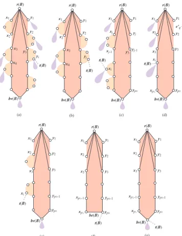
(4) Vol.2010-AL-129 No.5 2010/3/5 IPSJ SIG Technical Report r(B). 3.2 Tips of Rooted Blocks We define the “tip” t(B) of a block B as follows. If B consists of a single vertex u, then we define t(B) to be the vertex u. Otherwise, let {xi | i = 1, 2, . . . , pL } with pL = |V L (B)| (resp., {yj | j = 1, 2, . . . , pR } with pR = |V R (B)|) denote the set of vertices in the left (resp., right) side of B, where d(xi ) = d(r(B)) + i and d(yj ) = d(r(B)) + j. R R Case-1. Vcut (B) 6= ∅ (see Fig. 3(a)): Define t(B) to be the right vertex y ∈ Vcut (B) with the largest depth d(y). R R Case-2. Vcut (B) = ∅ and Vwing (B) 6= ∅ (see Fig. 3(b)): Define t(B) to be the right R wing-vertex y ∈ Vwing (B) with the largest depth d(y). R R L L Case-3. Vcut (B) = Vwing (B) = ∅ and Vcut (B) 6= ∅, where possibly Vwing (B) = ∅ L (see Fig. 3(c)-(d)): Define t(B) to be the left vertex x ∈ Vcut (B) with the largest depth d(x). R R L L Case-4. Vcut (B) = Vwing (B) = Vcut (B) = ∅ and Vwing (B) 6= ∅ (see Fig. 3(e)): L Define t(B) to be the left wing-vertex x ∈ Vwing (B) with the largest depth d(x). R R L L Case-5. |V (B)| = 2 or Vcut (B) = Vwing (B) = Vcut (B) = Vwing (B) = ∅, where possibly B(bv(B)) 6= ∅ (see Fig. 3(f)-(g)): Define t(B) to be the core-vertex u ∈ V ′ (B) with the largest depth d(u). Let t(B) be the right endvertex of be(B) if any. The spine of G is defined to be the sequence of all successors starting from the rightmost block B 1 ∈ B(rG ) by B 1 , B 2 , . . . , B p , where B 1 is the rightmost block in B(rG ), and each B i (i ≥ 2) is the rightmost block in B(t(B i−1 )) (Fig. 4). The tip t(G) of G is defined to be the tip t(B p ) of block B p , and the last block B p is called the tip-block of G.. y1. x1. r(B). r(B) x1. r(B) y1. x1. y1. y1. x1. e’q’ y2. x2. xj. y2 x2. x3. x3. y3. xj-1. yi x4. yj. y3. yj. x2. yj-1. x3. t(B). t(B) xi. t(B). ypR. bv(B). bv(B). (a). y2. y3. xi. (d). r(B). r(B). x2. x3. bv(B). (c). (b). y1. ypR-1. ypR. xpL. bv(B). r(B) x1. y3. xi. x4. t(B). y2. x1. y1. x2. y2. x3. y3. xpL-1. ypR-1. x1. y1. x2. y2. x3. y3. xpL-1. ypR-1. t(B) ypR. bv(B). xpL. be(B) t(B). ypR. xpL. ypR. bv(B) t(B). (e). Fig. 3. 4. Signatures of Embeddings. (f). (g). Tip t(B) of a rooted block B: (a) Case-1; (b) Case-2; (c) Case-3; (d) Case-3; (e) Case-4; (f) Case-5; and (d) Case-5.. the tip of G. We define the parent-embedding G′ = P (G) by removing the vertex u. Accordingly, G is called a child-embedding of G′ , which can be obtained from G′ by adding the vertex u. We first encode the operation that creates the vertex u into a sequence, denoted by γ(u). Then we define the signature σ(G) by the following recursive formula σ(G) = [σ(G′ ), γ(u)]. ′ ′ We set σ(G ) = ∅ if G is an empty graph.. This section will explain how to encode each colored and rooted outerplanar embedding into a sequence, called signature, such that each embedding can be uniquely reconstructed from its signature. We will first define a parent-child relationship between two outerplanar embeddings, and then introduce the signature for an outerplanar embedding based on its parent-embedding. Specifically, let G be an embedding with at least one vertex, and t(G) = u be. 4. c 2010 Information Processing Society of Japan.

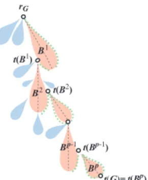
(5) Vol.2010-AL-129 No.5 2010/3/5 IPSJ SIG Technical Report. the vertices in V ′ (B) adjacent to u, and let d(v ′ ) ≥ d(v), where (v, v ′ ) is an edge ′ e in P (G), ( but (v, v ) can be an edge in B only when |V (B)| is even. Define (d(B), ∗, d(v ′ ), triangle, c(u)) if u, v and v ′ form a triangle in G γ(u) = (d(B), ∗, d(v ′ ), subdivide, c(u)) if v and v ′ are not adjacent in G. (P-3) Let u be a left wing-vertex of B: Let x and x′ be the two vertices in B ˜ adjacent(to u, where (x, x′ ) is an edge e in P (G) and e ∈ E(B) holds. Define L ′ (d(B), w , d(e), triangle, c(u)) if u, x and x form a triangle in G γ(u) = (d(B), wL , d(e), subdivide, c(u)) if x and x′ are not adjacent in G. (P-4) Let u be a right wing-vertex of B: Let y and y ′ be the two vertices in B ˜ adjacent(to u, where (y, y ′ ) is an edge e in P (G) and e ∈ E(B) holds. Define R ′ (d(B), w , d(e), triangle, c(u)) if u, y and y form a triangle in G γ(u) = (d(B), wR , d(e), subdivide, c(u)) if y and y ′ are not adjacent in G. By definition, we can see that each vertex code uniquely determines the resulting graph augmented with a new vertex. Let an element denote a vertex or an edge. In case (P-1) with h = 1, we say that G is obtained from P (G) by creating a new block at B with an application of γ(u) to vertex v = r(B) in P (G). In case (P-1) with h ≥ 2 and cases (P-2)-(P-4), we say that G is obtained from P (G) by expanding block B with an application of γ(u) to edge e in P (G). Such a vertex v and an edge e in P (G) are called applicable elements in P (G).. rG. t(B1). B1. B2. t(B2). B p-1 t(Bp-1) Bp. Fig. 4. t(G)= t(Bp). An illustration for a sequence of blocks between rG and t(G), which forms a spine.. Now we explain how to define the code γ(u) of the tip u of G. If u = tG , i.e., G consists of a single vertex rG , then we define the vertex code γ(u) = c(u) ∈ C. Otherwise, we define a vertex code γ(u) is a sequence (d1 (u), at(u), d2 (u), op(u), c(u)) of five entries such that d1 (u) and d2 (u) are nonnegative integers, c(u) ∈ C, at(u) ∈ {hL , wL , hR , wR , ∗}, and op(u) ∈ {new-block, star, triangle, subdivide}. Formally, we define the code γ(u) of the tip u of G as follows. Let B be the parent-block of u, which is the tip-block of G. (P-1) Let u be a head-vertex of B: Let h = |V ′ (B)|. If h = 1, i.e., B consists a leaf edge (v = r(B), u) of G, then for the block B ′ ′ ′ with v ∈ V  (B ), define ′ L ′   (d(B ), h , d(v), new-block, c(u)) if v is a left vertex of B ′ R γ(u) = (d(B ), h , d(v), new-block, c(u)) if v is a right vertex of B ′ (1)   (d(B ′ ), ∗, d(v), new-block, c(u)) otherwise, where B ′ = Br with d(Br ) = 0 if v = rG . If h = 2, i.e., B consists of a triangle (r(B), ℓv(B), u) of G and (r(B), ℓv(B)) is an edge in B, then define γ(u) = (d(B), ∗, d(ℓv(B)), triangle, c(u)). For h ≥ 3, let v and v ′ be the vertices in V ′ (B) adjacent to u, and let d(v ′ ) ≥ d(v), where (v, v ′ ) is an edge e in P (G). Define γ(u) = (d(B), ∗, d(v ′ ), star, c(u)). (P-2) Let u be an axial-vertex of B, where u is of degree 2 in G: Let v and v ′ be. 5. Canonical Embeddings We choose a specific embedding of a colored and rooted outerplanar graphs as canonical such that it facilitates identifying free symmetry at cut-vertices and reflectional symmetry along rooted blocks. We will explain the choice of canonical embedding after giving necessary notations. For two sequences A and B, let A > B mean that A is lexicographically larger then B, and let A ≥ B mean that A > B or A = B. Let A ⊐ B mean that B is a prefix of A and A 6= B, and let A ≫ B mean that A > B but B is not a prefix of A. Let A ⊒ B mean that A ⊐ B or A = B, i.e., B is a prefix of A. For two embeddings G1 and G2 of a graph H, we compare two signatures σ(G1 ) and σ(G2 ) by comparing their codes lexicographically code-wise. We compare two vertex codes γ and γ ′ by comparing their entries lexicographically, treating. 5. c 2010 Information Processing Society of Japan.

(6) Vol.2010-AL-129 No.5 2010/3/5 IPSJ SIG Technical Report. denote the sequence obtained from σcore (G(B); G) by eliminating the codes of right (resp., left) core-vertices and of the bottom vertex bv(B) (if any) after deleting the first four entries of each code in σcore (G(B); G), respectively. Thus, L R σcore (G(B); G) (resp., σcore (G(B); G)) is the sequence of color entries of left (resp., right) core-vertices of B. For each left wing-vertex u of B (resp., a child-vertex u ∈ Ch(v) of a vertex v in the left side of B), we define the flipped code γ(u) of vertex code γ(u) to be the code obtained from γ(u) by replacing the second entry wL (resp., hL ) with wR (resp., hR ). Symmetrically, for each right wing-vertex u of B (resp., a child-vertex u ∈ Ch(v) of a vertex v in the right side of B), we define the flipped code γ(u) of vertex code γ(u) to be the code obtained from γ(u) by replacing the second entry wR (resp., hR ) with wL (resp., hL ). For a notational convenience, we set γ(u) = γ(u) for the other vertices u ∈ V (G(B)) − {r(B)}. Let σL (G(B); G) (resp., σR (G(B); G)) denote the sequence obtained from σL (G(B); G) (resp., σR (G(B); G)) by replacing each vertex code γ(u) with γ(u). We can gain the following sufficient and necessary condition for left-sideheaviness at a rooted block. Lemma 2 An embedding G is left-side-heavy at a block B ∈ B(v) if and only L R if it holds [σcore (G(B); G), σL (G(B); G)] ≥ [σcore (G(B); G), σR (G(B); G)]. L L R For simplicity, denote σcore (G(B); G) by σcore . Similarly for σcore , σR and σL . We define the side-state  sd(B; G) of a block B in G as follows: L R   stc if “[σcore , σL ] ≫ [σcore , σR ]   nil if σ L = σ R and σ = ∅ R core core sd(B; G) = (3) L R  pfx if σcore = σcore and σL ⊐ σR 6= ∅    L R eqv if σcore = σcore and σL = σR 6= ∅. An embedding G is called canonical if it is left-sibling-heavy and left-side-heavy at all blocks in G. We find the following property of canonical embeddings. Lemma 3 Let G be an embedding of a colored and rooted outerplanar graph H. Then G is canonical if and only if σ(G) is lexicographically maximum among all σ(G′ ) of embeddings G′ ∈ ξ(H). Lemma 4 For a canonical embedding G with |V (G)| ≥ 2, its parentembedding P (G) is a canonical embedding. Family Tree Based on Lemma 4, we construct a rooted tree whose nodes. colors and labels as negative integers such that 0 > cK > cK−1 > · · · > c1 > ∗ > wL > hL > wR > hR > subdivide > triangle > star > new-block. For each block B ∈ B(v), the signature σ(G) of an embedding G contains a subsequence which consists of the codes of vertices in V (G(B)) − {v}, which we denote by σ(G(B); G). Left-sibling-heaviness An embedding G is called left-sibling-heavy at a block B ∈ B(v) = (B1 , B2 , . . . , Bp ) if B = B1 or σ(G) ≥ σ(G′ ) holds for the embedding G′ obtained from G by exchanging the order of Bi−1 and Bi = B in B(v). We can obtain the following result. Lemma 1 An embedding G is left-sibling-heavy at a block Bi ∈ B(v) = (B1 , B2 , . . . , Bp ) with i ≥ 2 if and only if σ(G(Bi−1 ); G) ≥ σ(G(Bi ); G) holds. ˆ ∈ B(r(B)) denote the sibling preceding B, where we let B ˆ = ∅ indicate Let B that there is no such sibling (i.e., B is the leftmost block in B(r(B))). We define the sibling-state sbl(B;  G) of a block B in G as follows: ˆ = ∅ or σ(G(B); ˆ G) ≫ σ(G(B); G)   stc if B ˆ 6= ∅ and σ(G(B); ˆ G) ⊐ σ(G(B); G) sbl(B; G) = (2) pfx if B   eqv if B ˆ 6= ∅ and σ(G(B); ˆ G) = σ(G(B); G). Left-side-heaviness An embedding G is called left-side-heavy at a block B ∈ B(v) if σ(G) ≥ σ(G′ ) holds for the embedding G′ obtained from G by replacing B with B f (thus flipping the embedding B along the axis through v and the bottom of B). The code subsequence σ(G(B); G) consists of six subsequences: the first consists of the codes of left or right core-vertices excluding bv(B) (denoted by σcore (G(B); G)), the second consists of the code of the descendants of the bottom vertex bv(B) if any (denoted by σb (G(B); G)), the third consists of the code of L left wing-vertices (denoted by σwing (G(B); G)), the fourth consists of the code of L descendants of left vertices (denoted by σdscd (G(B); G)), the fifth consists of the R code of right wing-vertices (denoted by σwing (G(B); G)), and the sixth consists R of the code of descendants of right vertices (denoted by σdscd (G(B); G)). Besides, let σL (G(B); G) (resp., σR (G(B); G)) denoted the subsequence L L of σ(G(B); G) consisting of σwing (G(B); G) and σdscd (G(B); G) (resp., R R L R σwing (G(B); G) and σdscd (G(B); G)). Let σcore (G(B); G) (resp., σcore (G(B); G)). 6. c 2010 Information Processing Society of Japan.

(7) Vol.2010-AL-129 No.5 2010/3/5 IPSJ SIG Technical Report. a code γ(uN +1 ) = (d1 , at, d2 , op, c) ∈ Γ(ε) to an element ε ∈ E(G). Let B h be the block in the spine with ε ∈ V ′ (B h ) ∪ E(B h ), i.e., the block to which a new vertex uN +1 is introduced, where B h is determined by d(B h ) = d1 . Let B ′ denote the new block created by γ(uN +1 ) (if ε is a vertex), where B ′ is the (h + 1)st block in the spine of G′ . Observe that G′ is also left-sibling-heavy and left-side-heavy at any block not in the spine of G or at any block B i with i > h in the spine of G. Thus, to know when G′ is canonical, we only need to examine states s1 , s2 , . . . , s2h−1 , s2h in G′ and the new sibling-state s2h+1 = sbl(B ′ ; G′ ) (if ε is a vertex) (recall that the side-state s2h+2 = sbl(B ′ ; G′ ) is always nil). We define copy-state cs(G) of G to be the state si∗ ∈ {eqv, pfx} with the minimum index i∗ in s(G), and the block B ℓ attaining si∗ = sbl(B ℓ ; G) or si∗ = sd(B ℓ ; G) is called the dominating block of G; let cs(G) = stc and i∗ = ∞ otherwise (i.e., each state in s(G) is stc or nil). Then we can characterize the element sequence E ∗ (G) by the copy-state cs(G) of G. Specifically, if cs(G) = stc, then E ∗ (G) = E(G), if cs(G) = eqv, then E ∗ (G) is the sequence of element obtained from E(G) by deleting the elements contained in a block B i with i ≥ ℓ in the spine, and if cs(G) = pfx, then E ∗ (G) is the sequence of elements obtained from E(G) by deleting the elements preceding a unique and specific element ε∗ (excluding ε∗ ), where ε∗ can be computed in O(1) time based on constant-size of the information about the dorminating block B ℓ of G. The vertex code set Γ = ∪ε∈E ∗ (G) Γ(ε).. represent canonical embeddings to be generated, called family tree, where the root-node is an empty graph, and other nodes are canonical embeddings of all colored and rooted outerplanar graphs. This family tree indicates that all colored and rooted outerplanar graphs may be generated by traversing all nodes in some order such as depth-first searching. 6. Generating Canonical Child-embeddings This section explains how to systematically generate all canonical childembddings from any given canonical embedding G without repetition and without testing duplication. Based on Sections 4 and 5, an embedding G′ is a canonical child-embedding of G if and only if G′ is obtained from G by attaching a new vertex v to an element ε (i.e., vertex or edge) in V (G) ∪ E(G) with a vertex code γ and G′ satisfies the left-heavy properties. The systematical generation of all canonical child-embeddings of G depends on the determination of all possible elements ε of G (arranged as a sequence E ∗ (G)) and all possible vertex codes (denoted by Γ). We can see that if all these valid elements and vertex codes can be automatically gained, then all canonical child-embeddings of G can be generated systematically without repetition. To obtain E ∗ (G) and Γ, we first identify all the elements ε in V ′ (B) ∪ E(B) and vertex code set Γ(ε) that admit a vertex code γ ∈ Γ(ε) such that G′ = G + γ(uN +1 ) remains left-side-heavy at a block B based on the same five cases used to define the tip of a block. We give the set of such elements in V ′ (B)∪E(B) as a sequence of these elements, called the element sequence E(B). Let E(B) = ∅ if sd(B; G) = eqv, since no application of γ(uN +1 ) is applied any element in V ′ (B) ∪ E(B) without violating left-side-heaviness of B. Then we identify the condition for G + γ(uN +1 ) to remain canonical, i.e., leftsibling-heavy and left-side-heavy at all blocks. For the spine B 1 , B 2 , . . . , B p of G, define sequences E(G) = [rG , E(B 1 ), E(B 2 ), . . . , E(B p )] and s(G) = [s1 = sbl(B 1 ; G), s2 = sd(B 1 ; G), s3 = sbl(B 2 ; G), s4 = sd(B 2 ; G), . . . , s2p−1 = sbl(B p ; G), s2p = sd(B p ; G)]. A canonical child-embedding G′ = G + γ(uN +1 ) of G is generated by applying. 7. Algorithm Recall that all canonical embeddings with at most n vertices to be enumerated are arranged in the family tree. Starting from a graph consisting of a single vertex, we recursively enumerate its first canonical child-embedding by appending a new vertex to the current graph until reaching an embedding that has no childembedding; and then backtracking to the most recent embedding which has childembeddings not being enumerated yet. Note that during the enumeration, we only output the constant-size difference between two consecutive embeddings. The above idea of enumeration is presented as the following Algorithm GENERATE, where “/*. . . */” indicates a comment. Algorithm GENERATE(n, C). 7. c 2010 Information Processing Society of Japan.

(8) Vol.2010-AL-129 No.5 2010/3/5 IPSJ SIG Technical Report. O(n) space.. Input: An integer n ≥ 1 and a set C = (c1 , c2 , . . . , cK ) of K colors. Output: All canonical embeddings of colored and rooted outerplanar graphs with at most n vertices. 1 begin 2 for each c ∈ C do 3 Let G be the graph consisting of a single vertex u1 (= rG ) with c(u1 ) = c; 4 Let Br be the imaginary parent-block of the root rG ; 5 Output c(u1 ) = c; 6 ε1 := u1 ; γ1 := (0, ∗, 0, new-block, c1 ); 7 GEN(G, Br , ε1 , γ1 ) 8 endfor 9 end. Given an embedding G with N vertices, a block B, an element ε ∈ E(B) and a code γ ∈ Γ(ε), Procedure GEN(G, B, ε, γ) recursively generates all descendantembeddings of G with at most n vertices, which is given as follows. Procedure GEN(G, B, ε, γ) /* Let N = |V (G)| ∈ [1, n − 1], and uN +1 be a new vertex that will be created. */ 1 begin 2 G′ :=Append(G, B, ε, γ); /* Compute a child-embedding G′ of G. */ 3 if N is odd then Output γ(uN +1 ) = γ endif; 4 if N + 1 < n then 5 ε1 := rG ; γ1 := (0, ∗, 0, new-block, c1 ); GEN(G′ , Br , ε1 , γ1 ) 6 endif; 7 if N is even then Output γ(uN +1 ) = γ endif; 8 RemoveTip(G′ ); /* Compute G from G′ by removing the tip of G′ . */ 9 [B ′ , ε′ , γ ′ ] :=NextCode(B, ε, γ; G); /* Calculate three parameters B ′ , ε′ and γ ′ to generate the next child-embedding of G */ 9 if [B ′ , ε′ , γ ′ ] 6= ∅ then GEN(G, B ′ , ε′ , γ ′ ) endif 10 end. Theorem 5 Given an integer n ≥ 1 and a set C = (c1 , c2 , . . . , cK ) of K ≥ 1 colors, the proposed algorithm enumerates all colored and rooted outerplanar graphs with at most n vertices without repetition in O(1) time per each and in. 8. Concluding Remarks This paper has proposed an efficient algorithm for generating all colored and rooted outerplanar graphs with at most given number n (≥ 1) vertices without repetition in O(1) time per each and O(n) space. References 1) Colbourn C. J. and Read R. C.: Orderly Algorithms for Graph Generation, International Journal of Computer Mathematics. Section A: Computer Systems: Theory, vol. 7, 167-172, 1979. 2) Fujiwara H., Wang J., Zhao L., Nagamochi H., and Akutsu T.: Enumerating Treelike Chemical Graphs with Given Path Frequency, Journal of Chemical Information and Modeling, vol. 48, pp. 1345-1357, 2008. 3) Georgii E., Dietmann S., Uno T., Pagel P., and Tsuda K.: Enumeration of Condition-dependent Dense Modules in Protein Interaction Networks, Bioinformatics, vol. 25, no. 7, pp. 933-940, 2009. 4) Goldberg L. A.: Polynomial Space Polynomial Delay Algorithms for Listing Families of Graphs, in proceedings of the twenty-fifth annual ACM symposium on Theory of computing, San Diego, California, United States, pp. 218-225, 1993. 5) Kawano S. and Nakano S.: Generating All Series-parallel Graphs, IEICE Transactions, vol. 88-A, no. 5, pp. 1129-1135, 2005. 6) Ishida Y., Zhao L., Nagamochi H., and Akutsu T.: Improved Algorithms for Enumerating Tree-like Chemical Graphs with Given Path Frequency, Genome Informatics, vol. 21, pp. 53-64, 2008. 7) Li G. and Ruskey F.: The Advantage of Forward Thinking in Generating Rooted and Free Trees, in Proceedings of the 10th Annual ACM-SIAM Symposium on Discrete Algorithms, pp. 939-940, 1999. 8) Nakano S. and Uno T.: Efficient Generation of Rooted Trees, NII Technical Report (NII-2003-005), 2003, available on http://research.nii.ac.jp/TechReports/03005E.html. 9) Nakano S. and Uno T.: Generating Colored Trees, Lecture Notes in Computer Science, vol. 3787, pp. 249-260, 2005. 10) Ruskey F. and Hu T. C.: Generating Binary Trees Lexicographically, SIAM Journal of Computing, vol. 6, pp. 745-758, 1977.. 8. c 2010 Information Processing Society of Japan.

(9)