The Effect of a Traffic Light on a Poisson Flow

THE EFFECT OF A TRAFFIC LIGHT ON A POISSON FLOW

TAKASI KISI AND KENJI HIYOSHI De/ense Academy

(Received June, 14, 1962) INTRODUCTION

Noncongested traffic flow is often taken as an example of a Poisson distribution, and in many cases this assumption is adopted in the pro-babilistic study of traffic flow to simplify its analysis.

If there is a bottleneck such as a traffic light or a toll gate, however, the flow near the bottleneck is by no means of Poisson type and we must go considerably down the stream to observe exponentially distributed time intervals between vehicles.

In this paper the following fictitious model of traffic flow is first investigated: Vehicles are stopped by a bottleneck, and released to move with constant time intervals. After the departure a car can travel with a constant desired speed, passing another car ahead being permitted. Thus the randomization of time intervals between successive vehicles is only caused by the distribution of desired speeds; the more down the stream, the more pefect randomization will be attained.

By means of both an elementary calculation in probability and the method of Monte Carlo, we obtain semiquantitative relations between the velocity distribution and the distance from the bottleneck where the flow can be regarded as Poisson from the practical point of view.

To verify the above relations. we made observations of the traffic flow through a highway connecting Tokyo with Osaka, and found that the number of passing vehicles per unit time didn't follow a Poisson di-stribution at a point 400 m distant from the traffic light, but at 1000 m point they did nearly, showing fairly good agreement with the above theoretical relations.

THEORETICAL CONSIDERATIONS

A flow which is obviously not of Poisson near a bottleneck seems to approach Poisson gradually as going down the road from the

Takasi KW, and Kenji Hi1l08hi

tleneck.

To investigate this manner, let us consider such an ideal flow or a model of traffic flow that vehicles leave a bottleneck continually with intervals, r, and travel down with constant desired speeds distributed uniformly as is

L----2.1V-~..:

v

speed

Fig. 1

shown in Fig. 1. (The average speed is V and the width LI V) Passing another vehicle ahead is assumed at will, and it is the only cause by wich randomization of intervehi-cular spacing is attained.

Under these assumptions an elemen-tary calculation in probability yields the following result:

re

If D~~ 2L1V-' ( l )

and D~rV, (2)

then the probability that a vehicle reaches a point at a distance D from the bottleneck in the time interval (t, t+Llt) is independent of both t and the arrival of other vehicles and

p=,;=Jt. (3')

r

This means tha ttime intervals between passing vehicles through the point have an exponential distribution, in other \vords, the number of passing vehicles in a certain time interval has a Poisson distribution.

For the sake of another approach, we examine the same problem by means of the method of Monte Carlo. Numerical values adopted in this case is

::-=4 sec: V= 10 m/sec; LI V=2, 4, 5, 8 m/sec

and the calculation is carried out with the following procedure. Using a table of random numbers, the speed of each vehicle is determined, their time-spatial trajectories are drawn in a section paper, and then time in-tervals between vehicles passing through a point at an arbitrary distance can be easily obtained. xLtest with a confidence level 0.10 is used to test whether the time intervals have an exponential distribution or not since the sample size is rather small. For convenience, if calculated ;(-value is not significant, the distribution is considered as exponential.

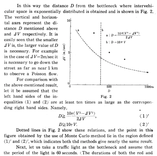
The Effect of a Traffic Light on a Poisson Flow 690 In this way the distance D from the bottleneck where intervehi-cular space is exponentially distributed is obtained and is shown in Fig. 2._ The vertical and horizon·

tal axes represent the di· stance D mentioned above and £1 V respectively. It is easily seen that the smaller £1 V is, the larger value of D is necessary. For example in the case of £1 V=2m/sec it is necessary to go down the street as far as near 1 km to observe a Poisson flow.

10 I I I I I I 'D_lO'I'(V'-jV') a. - 2jV b:D=lO'I'V

---

---For comparison with the above-mentioned result, let it be assumed that the

o ---"-__ ' _~_.-L

o --5""'OO;;--~-~--'--~~lOO'Om,

D left hand sides of the in- Fig. 2

equalities (1) and (2)' are at least ten times as large as the correspon-ding right hand sides. Namely,

D> 10~!,"~:-£1 V2)

= 2£1 V '

D~10,V.

(1)' (2 )'

Dotted lines in Fig. 2 show these relations, and the point in this. figure obtained by the use of Monte Carlo method lie in the region defined (1), and (2)" which indicates both thd methods give nearly the same result. Next, let us take a traffic light as the bottleneck and assume that the period of the light is 60 seconds. (. The durations of both the red and the green are 30 sec.) During the red, vehicles are stopped and when the light turns green. they begin to start continually with fonstant time in-tervals 5 sec. and travel down the street with desired speeds. (It corres-ponds to the traffic volume 420 vehicles per an hour.)

As to the velocity distribution, let us adopt V=lO 1; and £1V=2:

m/sec (the standard deviation is 1.2 m/sec) which are good approxir~a­ tions to the values observed in the actual case stated below. In the actual situation, however, the distribution is not uniform, and it should be no-ticed that the above model is nothing but a simplified one to obtain a

10 TaktBt KiIII and Kenji Htgmdai

rough estimation.

Monte Carlo method is applied in the same way as before, and the

O.4r

O'3~!

-

~ O.2~

..

°O~i ---,----n----~--~~--.~

3

number of vehicle per 13 sec.

Fig. 3

vehicle counts in an interval 13 sec are obtained. The co-unting distributions at points about 300 m and 1 km from the traffic light are shown in Fig. 3 in comparison with a Poiss on distribution. The for-mer largely deviates from the Poiss on distribution, but the latter can be regarded as

n Poisson according to the rule

based on XL test mentioned above.

MEASUREMENTS AND RESULTS

To verify the results obtained by the mathematical considerations, ·obsenations of traffic flow were carried out both in Fujisawa and in Yokosuka.

In Fujisawa, the width of the national highway connecting Tokyo with Osaka is about 11 m, and the road is not so curved that passing another vihicle ahead is easily done. At an intersection in the western part of the city a traffic light is operating, and there are neither traffic lights nor intersections within a considerable distance to the west of this point. If the observation is made as to the traffic flow in the lane for 'Osaka, these situations are suitable for our experiment.

The period of the light is 63 sec in which the durations of the red, .green, and amber are 26, 23, 4 sec. respectively.

The speed of each vehicle is measured with a pen recorder by re-cording the time of passing two points which are 50 m apart, and this .enanble us to count the number of passing vehicles per 15 sec. too.

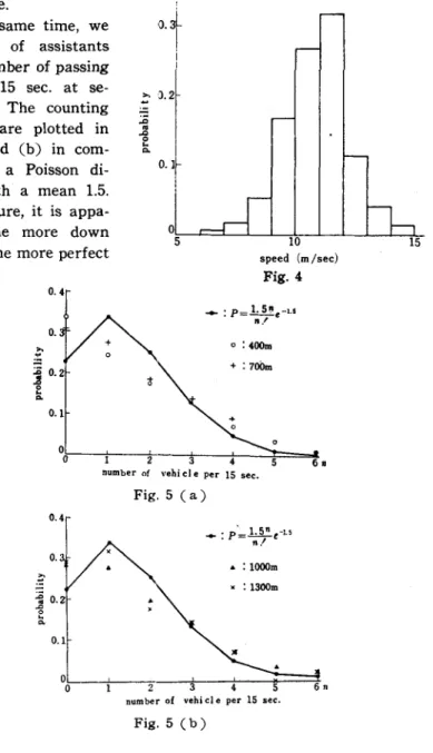
The speed distribution observed at a point about 700 m from the traffic light is shown in Fig. 4, and the mean and the standard deviation is calculated as 11 m/sec and 1.4 m/sec respectively. The traffic volume is .350 vehicles per an hour, which corresponds to l.5 vehicles per 15 sec.

The Effect of a Traffic Light 011 a Poi.80ft Flow

in the average.

At the same time, we make a few of assistants count the number of passing vehicles per 15 sec. at se-veral points. The counting distributions are plotted in Fig. 5 Ca) and Cb) in com-parison with a Poisson di-stribution with a mean 1.5.

From this figure, it is appa-rent that the more down the stream, the more perfect

0.4 o. 10 speed (m/sec) Fig. 4 o :400m + : 700m 6.

number of vehi cl e per 15 sec.

Fig. 5 Ca) 0.4 0.1 ... : p'= 1.5,n e-L5 n . • : 1000m : 1300m o~~ __ ~. __ ~ __

-+ __

number of vehi cl e per 15 sec.

Fig. 5 Cb)

Takaal KiBi and KenJi Ht1/Oshi

randomization is attained, and that Poisson flow IS observed, as was

expected at a point about 1 km or more distant from the traffic light. To illustrate that passing another car ahead plays an important roie in randomization of intervehicular space, let us present a counting distribution observed in a region where passing another car ahead is prohibited. 0.4 0.3 0.1 o : P=o 1.5ne-1. 5

n'

number of vehi cl e per 15 sec.

Fig. 6

In Fig. 6 an observed distribution at 2000 m point is shown, which apparently deviates from the Poisson distribution.

In the similar way another observation was carried out in Yoko-suka. A straight stretch of a highway with width 15 m suitable for our

0.3 '" .-::: 0.2' O. 1 O~~~-L~~~~-L~ __ L-~~~ 5 10 speed (m/sec) Fig. 7

The Effect of a Traffic Liglat 011 a p e ; -Ft- 73

observation is chosen. The period of the traffic light is 52 sec. (the dura-tions of the red, green, and amber are 22, 25, and 5 sec. respectively). The speed distribution observed at 500 m point has a mean 11 m/sec and a standard deviation 1.7 m/sec as is shown in Fig. 7. The traffic volume is 410 vehicles per an hour or 1.7 vehicles per 15 sec.

The counting distributions obtained at 500 m and I()()() m point are 0.4

6 .. number of v.hi cl e per 15 sec.

Fig. 8

plotted in Fig. 8, and a Poisson distribution with a mean 1.7 is plotted for the comparison's sake, too. The observed values at I()()() m point do not deviate much from the Poisson distribution, which is similar to the former case.

CONCLUSION

From these considerations we can conClude that under such circum-stances (traffic volume, road conditions, velocity distributions, etc.) as treated in the preceding paragraph, a traffic light does not effect on the intervehicular space over a distance 1 km or so, and that the traffic flow there may be treated as a Poisson flow.