2003, Vol. 46, No. 3, 319-341
STATIONARY QUEUE LENGTH IN A FIFO SINGLE SERVER QUEUE WITH SERVICE INTERRUPTIONS AND MULTIPLE BATCH
MARKOVIAN ARRIVAL STREAMS
Hiroyuki Masuyama Tetsuya Takine Kyoto University
(Received September 2, 2002)
Abstract This paper considers a FIFO single-server queue with service interruptions and multiple batch Markovian arrival streams. The server state (on and off), the type of arriving customers and their batch size are assumed to be governed by a continuous-time Markov chain with finite states. To put it more concretely, the marginal process of the server state is a phase-type alternating Markov renewal process, the marginal arrival process is a batch marked Markovian arrival process, and they may be correlated. Further, service times of arriving customers are allowed to depend on both their arrival stream and the server state on arrival. For such a queue, we derive the vector joint generating function of the numbers of customers from respective arrival streams. Further assuming discrete phase-type batch size distributions, we establish a numerical algorithm to compute the joint queue length distribution at a random point in time. Finally, we show some numerical examples and examine the impact of system parameters on the queue length distribution.
Keywords: Queue, batch marked MAP, FIFO, service interruptions
1. Introduction
This paper considers a FIFO single-server queue with service interruptions. In such a queue, the state of the server changes on and off alternately. While in on-state, the server is available for service. On the other hand, while in off-state, the server dose not work even if customers are present in the system. Hereafter periods during which the server is in on-state (resp. off-state) are called on-periods (resp. off-periods).
Queues with service interruptions have many applications in the fields of manufacturing, computer and telecommunications systems, and many studies on those queues have been done for a few decades. A detailed survey on queues with service interruptions can be found in the introduction of the paper by Federgruen and Green [1]. They mainly discussed approximation methods for an M/G/1 queue with service interruptions, where on- and off-periods are generally distributed [1]. Further, assuming a phase-type on-period distribution, they established an exact algorithm to compute the steady-state queue length distribution [2].
Recently, more general queues with service interruptions have been studied. Sengupta [9] considered the model where on- and off-period distributions are general, customers arrive according to a Poisson process whose arrival rate depends on the server state, and service times are generally distributed, depending on the server state upon arrival. He showed that the amount of unfinished work in such a queue is closely related to the waiting time in a special GI/G/1 queue. Also, Takine and Sengupta [12] considered a single-server queue with
service interruptions, where both the server state and arrival processes are governed by a finite-state Markov chain. Namely, the marginal processes of the server state and customer arrivals form an alternating phase-type Markov renewal process and a MAP (Markovian arrival process) [5], respectively, and they may be dependent. For this queue, they obtained the steady-state queue length distribution. The crucial assumption posed in [12] was i.i.d. (independent and identically distributed) service times.
This paper considers an extension of the results in [12] to allowing multiple batch Marko-vian arrival streams. Thus, the marginal arrival process follows a batch marked MAP [3, 4, 6]. Further, service times of customers can depends on both their arrival stream and the server state on arrival. As stated in [12], such a queue cannot be analyzed by the conventional M/G/1 paradigm [8]. To analyze the extended model, therefore, we use a new approach developed in [7, 13–15], which is based on the invariant relationship of the joint queue length distributions at random points in time and at departures [14]. We then derive the vector joint generating function of the numbers of customers from respective arrival streams. Further assuming discrete phase-type batch size distributions as in [7], we provide a computational algorithm for the steady-state joint queue length distribution. We also show some numerical examples and examine the impact of system parameters on the queue length distribution.
The rest of this paper is divided into four sections. In section 2, the mathematical model is described. Section 3 briefly discusses the sojourn time distribution. In section 4, we first derive a general formula for the joint queue length distribution, and assuming discrete phase-type batch size distributions, we show recursive formulas to compute the joint queue length distribution. Finally, in section 5, we show some numerical examples. Throughout the paper, matrices and vectors are denoted by bold capital letters and bold small letters, respectively, and the empty sum is defined as zero.
2. Model
We consider a FIFO single-server queue with service interruptions. The state of the server changes on and off alternately, and while the server is being on, customers are served suc-cessively. On the other hand, services of customers stop temporally while the server is being off, and interrupted services are restarted in a preemptive-resume manner when the server becomes on again. In what follows, we call the process of the server state the on-off process. We assume that both the on-off and arrival processes are governed by an underlying finite-state Markov chain that is assumed to be irreducible. Let M = {1, . . . , M } denote the state space of the underlying Markov chain, where M ≥ 2. It stays in state i (i ∈ M) for an exponential interval of time with mean µ−1
i , and when the sojourn time in state i
has elapsed, the underlying Markov chain changes its state to state j with probability σi,j
(j ∈ M), where
X
j∈M
σi,j = 1.
The on-off process of the server is defined in the following way. The state space M is divided into two disjoint sub-spaces, Mon = {1, . . . , Mon} and Moff = {Mon+ 1, . . . , Mon+ Moff}, where Mon ≥ 1, Moff ≥ 1 and Mon+ Moff = M. The server is assumed to be on (resp.
off) while the underlying Markov chain is being in state i ∈ Mon (resp. i ∈ Moff). Thus
the on-off process forms a phase-type alternating Markov renewal process.
Next we describe the arrival process of customers. We assume that there are K (K ≥ 1) arrival streams. Let K denote a set of class indices, i.e., K = {1, . . . , K}. Customers arriving
from the kth (k ∈ K) arrival stream are called class k customers. Given a state transition of the underlying Markov chain from state i to state j (i, j ∈ M), n (n = 1, 2, . . .) customers of class k (k ∈ K) arrive in batch with probability σk,i,j(n)/σi,j, where
X k∈K ∞ X n=1 σk,i,j(n) ≤ σi,j,
for all i, j ∈ M. Note that customers in the same batch belong to the same class. For later use, we define σi,j(0) (i, j ∈ M) as
σi,j(0) = σi,j − X k∈K ∞ X n=1 σk,i,j(n).
Note that σi,j(0)/σi,j represents the conditional probability of no arrivals given that a state
transition from state i to state j happens. Without loss of generality, we assume σi,i(0) = 0
for all i (i ∈ M).
In terms of service times, class k customers are further classified into two sub-classes based on the server state on arrival. We call class k customers arriving in on-periods (resp. off-periods) class on (resp. off) customers. Service times of class on (resp. k-off) customers are assumed to be i.i.d. according to a distribution function Hk,on(x) (resp.
Hk,off(x)) with finite mean hk,on (resp. hk,off).
In the rest of this paper, we impose two assumptions on σk,i,j(n). For each k (k ∈ K),
there exists at least one triad (i, j, n) (i, j ∈ M, n = 1, 2, . . .) such that σk,i,j(n) > 0. Thus
arrivals of class k customers are certain. Further σk,i,j(n) = 0 (k ∈ K) if i ∈ Mon and j ∈ Moff or if i ∈ Moff and j ∈ Mon. Thus arrivals of customers and changes of the server
state never happen simultaneously.
We now introduce some notations. Let C denote an M × M matrix whose (i, j)th (i, j ∈ M) element Ci,j is given by
Ci,j =
(
−µi, if i = j,
σi,j(0)µi, otherwise.
For each k ∈ K, let Dk(n) (n = 1, 2, . . .) denote an M × M matrix whose (i, j)th (i, j ∈ M)
element Dk,i,j(n) is given by
Dk,i,j(n) =
(
σk,i,j(n)µi, if i, j ∈ Mon or i, j ∈ Moff,
0, otherwise.
Then the on-off and arrival processes are characterized by C and Dk(n) (k ∈ K, n =
1, 2, . . .). Note here that C and Dk(n) have the following structure:
C = " Con Eon,off Eoff,on Coff # , Dk(n) = " Dk,on(n) O O Dk,off(n) # ,
where Con and Dk,on(n) are Mon×Mon matrices, Coff and Dk,off(n) are Moff×Moff matrices,
and Eon,off and Eoff,on are Mon× Moff and Moff× Mon matrices, respectively.
We define Dk,ξ (k ∈ K, ξ = on, off) and Dξ (ξ = on, off) as
Dk,ξ = ∞ X n=1 Dk,ξ(n), Dξ = X k∈K Dk,ξ,
respectively. We also define D as D = " Don O O Doff # .
Note that the infinitesimal generator of the underlying Markov chain is given by C + D. Note also that (C + D)e = 0, where e denotes a column vector whose elements are all equal to one. We denote the stationary probability vector of the underlying Markov chain by π. Because of the finite state space M and the irreducibility of the underlying Markov chain,
π is uniquely determined so as to satisfy π(C + D) = 0 and πe = 1. Let πon (resp. πoff)
denote a 1 × Mon (resp. 1 × Moff) vector representing the conditional stationary probability
vector of the underlying Markov chain given that the server is on (resp. off). Note that πon
and πoff satisfy πon · Con + Don+ Eon,off h −Coff − Doff i−1 Eoff,on ¸ = 0, πone = 1, πoff ·
Coff + Doff+ Eoff,on
h −Con− Don i−1 Eon,off ¸ = 0, πoffe = 1,
respectively. Let ron and roff denote fractions of time being in on- and off-periods,
respec-tively. We then have
ron = Ion Ion+ Ioff , roff = Ioff Ion+ Ioff ,
where Ion and Ioff denote the mean lengths of on- and off-periods, respectively, and they
are given by Ion = πoffEoff,on πoffEoff,one h −Con− Don i−1 e, Ioff = πonEon,off πonEon,offe h −Coff− Doff i−1 e.
Note here that π, πon and πoff are related by
π = (ronπon, roffπoff).
We denote the mean arrival rate of class k (k ∈ K) customers during on- (resp. off-) periods by λk,on (resp. λk,off):
λk,ξ = πξ ∞
X
n=1
nDk,ξ(n)e, ξ = on, off.
Let λk= ronλk,on+ roffλk,off (k ∈ K) denote the mean arrival rate of class k customers. We
define ρ as the offered load, i.e.,
ρ = ron
X
k∈K
λk,onhk,on+ roff
X
k∈K
λk,offhk,off.
Further, we define ρon as the conditional utilization factor given that the server is on, which
is given by
ρon = ron−1ρ.
3. Sojourn Time
This section considers sojourn time. Because sojourn time is closely related to the amount of unfinished work in the system, we first discuss the latter.
Let V and S denote generic random variables representing the amount of unfinished work and the state of the underlying Markov chain, respectively, in steady state. With these, we define v(x) as a 1 × M vector whose jth element represents Pr[V ≤ x, S = j]. Further we define vξ(x) (ξ = on, off) as a 1 × Mξ vector whose jth element represents
Pr[V ≤ x, S = j | S ∈ Mξ]. Note here that v(x) is given in terms of von(x) and voff(x): v(x) = (ronvon(x), roffvoff(x)).
Thus, we consider von(x) and voff(x) below.
Let Joff,on(x) denote an Moff× Mon matrix whose (i, j)th element represents the
proba-bility that the amount of work arriving during an off-period is not greater than x and the underlying Markov chain is in state j ∈ Mon at the beginning of the next on-period, given
that the off-period starts in state i ∈ Moff. We define Dξ(x) (ξ = on, off) as
Dξ(x) = X k∈K ∞ X n=1 Dk,ξ(n)Hk,ξ(n)(x),
where Hk,ξ(1)(x) = Hk,ξ(x) and Hk,ξ(n)(x) (n = 2, 3, . . .) denotes the n-fold convolution of Hk,ξ(x)
with itself. According to [10], we define an Mon × Mon matrix Qon as an infinitesimal
generator of the irreducible Markov chain obtained by observing the underlying Markov chain only when the system is idle in on-periods. Note that Qon satisfies
Qon = Con+
Z ∞
0 dDon(x) exp(Qonx) + Eon,off
Z ∞
0 dJoff,on(x) exp(Qonx).
Because ρon < 1, Qon is uniquely determined by the above equation [10]. Let κon denote a
probability vector satisfying κonQon = 0. Then, von(0) is given by [10] von(0) = (1 − ρon)κon. Further, the LST v∗ on(s) of von(x) satisfies [10] v∗ on(s) · sI + Con+ D∗on(s) + Eon,off h −Coff − D∗off(s) i−1 Eoff,on ¸ = s(1 − ρon)κon, (3.1)
where D∗ξ(s) (ξ = on, off) denotes the LST of Dξ(x) and I(m) denotes an m × m identity
matrix. We suppress the size m when it is clear from the context. As for the LST v∗
off(s) of voff(x), using the same approach as in [12], we readily obtain
v∗ off(s) = v∗ on(s)Eon,off πonEon,offe [−Coff− D∗off(s)]−1 Ioff . (3.2)
Next we analyze sojourn time. To do so, we first consider completion time, which is a time interval from the beginning of a service to its completion, including service interruptions. Let Tc(u) denote a generic random variable representing the completion time of a service
of u units. Note that the completion time Tc(u) depends on the state of the underlying
Markov chain at the beginning of the service, as well as the amount of the service. We assume that a service commences at time 0, and let St denote the state of the underlying
Markov chain at time t. We denote the number of class k (k ∈ K) customers arriving in interval (0, t] by Lk(t). We then define P∗∗(z, s | u) as an Mon× Mon matrix whose (i, j)th
element represents E Y k∈K zLk(Tc(u))
k exp(−sTc(u)) 1{STc(u) = j ∈ Mon} | S0 = i ∈ Mon
,
where z denotes a 1×K complex vector (z1, . . . , zK) and 1{χ} denotes an indicator function
of event χ. Further, we define D∗
k,ξ(zk) (k ∈ K, ξ = on, off) as D∗k,ξ(zk) = ∞ X n=1 zn kDk,ξ(n). (3.3)
Following an approach similar to [12], we obtain
P∗∗(z, s | u) = exp [K(z, s)u] , where K(z, s) = Con+ X k∈K D∗ k,on(zk) − sI + Eon,off sI − Coff −X k∈K D∗ k,off(zk) −1 Eoff,on.
We are now ready to discuss sojourn time.
Let Wk (k ∈ K) (resp. Wk,ξ (k ∈ K, ξ = on, off)) denote a generic random variable
representing the sojourn time of a class k (resp. k-ξ) customer. Also let Wk,ξ(n; m) (k ∈ K,
ξ = on, off, n = 1, 2, . . ., m = 1, . . . , n) denote a generic random variable representing the
sojourn time of a randomly chosen class k-ξ customer who is a member of a batch of size
n and the mth served customer among members in the same batch. For convenience, we
assume that if λk,ξ = 0, Wk,ξ = 0, and if Dk,ξ(n) = O for some n (n ≥ 1), Wk,ξ(n; m) = 0
for all m (m = 1, . . . , n). Further, let w∗
k(s), wk,ξ∗ (s) and w∗k,ξ(s | n; m) denote the LSTs
of the distributions of Wk, Wk,ξ and Wk,ξ(n; m), respectively. Because a randomly chosen
departing customer of class k (k ∈ K) belongs to class k-ξ (ξ = on, off) with probability
rξλk,ξ/λk, we obtain w∗ k(s) = ronλk,on λk w∗ k,on(s) + roffλk,off λk w∗ k,off(s).
Note here that
w∗ k,ξ(s) = ∞ X n=1 nπξDk,ξ(n)e λk,ξ · 1 n n X m=1 w∗ k,ξ(s | n; m), k ∈ K, ξ = on, off, (3.4)
if λk,ξ > 0, and otherwise wk,ξ∗ (s) = 1. Thus, in what follows, we consider wk,ξ∗ (s | n; m)
(k ∈ K, ξ = on, off, n = 1, 2, . . ., m = 1, . . . , n).
Let Hk,ξ(n; m) (k ∈ K, ξ = on, off, n = 1, 2, . . ., m = 1, . . . , n) denote a generic random
variable representing the service time of a randomly chosen class k-ξ customer who is a member of a batch of size n and the mth served customer among members of the same batch. Because Wk,ξ(n; m) = Wk,ξ(n; 1) +
Pm
and m = 1, . . . , n, we obtain for n = 1, 2, . . . and m = 1, . . . , n,
w∗
k,on(s | n; m) =
1
πonDk,on(n)e
Z ∞
0 dvon(x)Dk,on(n) exp [Ω(s)x] ·
·Z ∞
0 dHk,on(y) exp [Ω(s)y]
¸m
e, (3.5)
w∗k,off(s | n; m) = 1
πoffDk,off(n)e
Z ∞
0 dvoff(x)Dk,off(n)
h
sI − Coff− Doff
i−1
·Eoff,onexp [Ω(s)x]
·Z ∞
0 dHk,off(y) exp [Ω(s)y]
¸m
e, (3.6) respectively, where Ω(s) = K(1, . . . , 1, s). Note here that the (i, j)th (i, j ∈ Mon) element
of exp[Ω(s)x] represents E[exp(−sTc(x))1{STc(x) = j} | a service of x units starts at time 0
and S0 = i]. Thus from (3.4) and (3.5), we obtain for k ∈ K, w∗ k,on(s) = 1 λk,on ∞ X n=1 Z ∞ 0 dvon(x)Dk,on(n) exp [Ω(s)x] n X m=1 ·Z ∞
0 dHk,on(y) exp [Ω(s)y]
¸m
e,
if λk,on > 0, and otherwise w∗k,on(s) = 1. Similarly, from (3.4) and (3.6), we obtain for k ∈ K,
w∗ k,off(s) = 1 λk,off ∞ X n=1 Z ∞ 0 dvoff(x)Dk,off(n) h sI − Coff − Doff i−1 Eoff,onexp [Ω(s)x] · n X m=1 ·Z ∞
0 dHk,off(y) exp [Ω(s)y]
¸m
e,
if λk,off > 0, and otherwise wk,off∗ (s) = 1.
4. Joint Queue Length Distribution
This section considers the joint queue length distribution. Let Nk (k ∈ K) denote a generic
random variable representing the number of class k customers in the stationary system. We then define p(n) (n ∈ Z) as a 1 × M vector whose jth element represents Pr[N1 = n1, . . ., NK = nK, S = j], where n denotes a 1 × K nonnegative integer vector (n1, . . . , nK) and
Z = {(n1, . . . , nK) ; nk = 0, 1, . . . for all k ∈ K}. Further, let Nν(Dk) (k, ν ∈ K) and S(Dk)
(k ∈ K) denote generic random variables that represent the number of class ν customers in the system and the state of the underlying Markov chain, respectively, immediately after departures of class k customers in steady state. We then define qk(n) (k ∈ K, n ∈ Z) as a 1 × M vector whose jth element represents Pr[N(Dk)
1 = n1, . . . , NK(Dk) = nK, S(Dk) = j].
Applying Theorem 1 in [14] to our model, we have the following theorem. Theorem 4.1 ([14]) The p(n) (n ∈ Z) is recursively determined by
p(0) = X k∈K λkqk(0)(−C)−1, p(n) = X k∈K λk(q k(n) − qk(n − ek)) + nk X mk=1 p(n − mkek)Dk(mk) (−C)−1, n ∈ Z+, where Z+ = Z − {0}, q
k(n) = 0 for n ∈/ Z and ek (k ∈ K) denotes the kth unit vector:
ek= (0, . . . , 0, 1
kth
, 0, . . . , 0).
Thus the p(n) is given in terms of the qk(n). We then consider the qk(n) in section 4.1. Further, in section 4.2, assuming discrete phase-type batch size distributions, we derive numerically feasible recursions for some quantities required in computing the qk(n).
4.1. Joint queue length distribution immediately after departures We define q∗
k(z) (k ∈ K) as the vector generating function of the joint queue length
distri-bution immediately after departures of class k customers.
q∗k(z) = X
n∈Z
zn1
1 · · · zKnKqk(n), |zk| ≤ 1 for all k ∈ K.
Let N(Dk,ξ)
ν and S(Dk,ξ)(k, ν ∈ K, ξ = on, off) denote generic random variables that represent
the number of class ν customers in the system and the state of the underlying Markov chain, respectively, immediately after departures of class k-ξ customers in steady state. We define qk,ξ(n) (k ∈ K, ξ = on, off) as a 1 × Mon vector whose jth element represents
Pr[N(Dk,ξ)
1 = n1, . . . , NK(Dk,ξ) = nK, S(Dk,ξ) = j]. We also define q∗k,ξ(z) (k ∈ K, ξ = on, off)
as q∗k,ξ(z) = X n∈Z zn1 1 · · · zKnKqk,ξ(n). We then have q∗ k(z) = Ã ronλk,on λk q∗ k,on(z) + roffλk,off λk q∗ k,off(z), 0, . . . , 0 ! , (4.1)
because all departures always occur in on-periods. In the rest of this subsection, we derive q∗
k,on(z) and q∗k,off(z). We call a randomly chosen
class k-ξ (k ∈ K, ξ = on, off) customer who is a member of a batch of size n and the mth served customer among members in the same batch the tagged customer. Further we call the batch to which the tagged customer belongs the tagged batch. Let N(Dk,ξ)
ν (n; m) and
S(Dk,ξ)(n; m) (k, ν ∈ K, ξ = on, off, n = 1, 2 . . ., m = 1, . . . , n) denote generic random
variables that represent the number of class ν customers in the system and the state of the underlying Markov chain, respectively, immediately after the departure of the tagged customer. We then define q∗
k,ξ(z | n; m) (k ∈ K, ξ = on, off, n = 1, 2 . . ., m = 1, . . . , n) as a
1 × Mon vector whose jth element represents E
h Q ν∈KzN (Dk,ξ) ν (n;m) ν 1{S(Dk,ξ)(n; m) = j} i . It is easy to see that q∗
k,ξ(z) can be written in terms of q∗k,ξ(z | n; m):
q∗k,ξ(z) = ∞ X n=1 nπξDk,ξ(n)e λk,ξ 1 n n X m=1 q∗k,ξ(z | n; m), k ∈ K, ξ = on, off, (4.2) if λk,ξ > 0, and otherwise q∗k,ξ(z) = 0.
Note here that customers who contribute to q∗
k,on(z | n; m) can be divided into three
types: (i) customers arriving during the completion time of the total unfinished work im-mediately before the arrival of the tagged batch, (ii) customers arriving during an interval from the beginning of the first service of a member in the tagged batch to the completion of the service of the tagged customer, and (iii) n − m customers who belong to the tagged batch and receive their services after the tagged customer. It then follows that for k ∈ K,
n = 1, 2, . . . and m = 1, . . . , n, q∗ k,on(z | n; m) = zkn−m· Z ∞ 0 dvon(x)Dk,on(n)N∗(z | x) πonDk,on(n)e · ·Z ∞ 0 dHk,on(y)N ∗(z | y)¸m, (4.3) where N∗(z | x) = P∗∗(z, 0 | x), i.e., N∗(z | x) = exp Con+ X k∈K D∗ k,on(zk) + Eon,off −Coff − X k∈K D∗ k,off(zk) −1 Eoff,on x . (4.4)
Note that N∗(z | x) denotes the matrix joint generating function for the numbers of arrivals
in respective classes during the completion time of a service of x units. Similarly, we have for k ∈ K, n = 1, 2, . . . and m = 1, . . . , n, q∗ k,off(z | n; m) = zn−mk · Z ∞ 0 dvoff(x)Dk,off(n)
πoffDk,off(n)e
−Coff −X k∈K D∗ k,off(zk) −1 Eoff,onN∗(z | x) · ·Z ∞ 0 dHk,off(y)N ∗(z | y) ¸m . (4.5)
Thus, from (4.2), (4.3) and (4.5), we obtain the following theorem. Theorem 4.2 q∗ k,on(z) (k ∈ K) is given by q∗ k,on(z) = 1 λk,on ∞ X m=1 ∞ X l=0 zl k Z ∞ 0 dvon(x)Dk,on(m + l)N ∗(z | x)·Z ∞ 0 dHk,on(y)N ∗(z | y)¸m,
if λk,on > 0, and otherwise q∗k,on(z) = 0. On the other hand, q∗k,off(z) (k ∈ K) is given by
q∗ k,off(z) = 1 λk,off ∞ X m=1 ∞ X l=0 zl k Z ∞ 0 dvoff(x)Dk,off(m + l) −Coff− X k∈K D∗ k,off(zk) −1 Eoff,on ·N∗(z | x) ·Z ∞ 0 dHk,off(y)N ∗(z | y) ¸m , if λk,off > 0, and otherwise q∗k,off(z) = 0.
4.2. Recursions for models with discrete phase-type batch sizes
In this subsection, we develop recursive formulas to compute the joint queue length distribu-tion qk(n) immediately after departures of class k customers under the following assumption. Assumption 4.1 Batch sizes of class k-ξ (k ∈ K, ξ = on, off) are independent of the state
of the underlying Markov chain and i.i.d. according to a discrete phase-type distribution with representation (αk,ξ, Pk,ξ), where αk,ξ denotes a 1 × Mk,ξ probability vector and Pk,ξ
denotes an Mk,ξ × Mk,ξ substochastic matrix.
Under Assumption 4.1, Dk,ξ(n) (k ∈ K, ξ = on, off) is given by
Dk,ξ(n) = gk,ξ(n)Dk,ξ, n = 1, 2, . . . ,
where gk,ξ(n) denotes the probability mass function of the batch size of class k-ξ:
gk,ξ(n) = αk,ξPn−1k,ξ (I − Pk,ξ)e, n = 1, 2, . . . .
Thus, Theorem 4.2 is reduced to:
Corollary 4.1 Under Assumption 4.1, q∗
k,on(z) (k ∈ K) is given by q∗k,on(z) = 1 λk,on Z ∞ 0 dvon(x)Dk,onN ∗(z | x) · µ αk,on⊗ Z ∞ 0 dHk,on(y)N ∗(z | y) ¶ · I − Pk,on⊗ Z ∞ 0 dHk,on(y)N ∗(z | y) ¸−1 ·hn(I − zkPk,on)−1(I − Pk,on)e o ⊗ I(Mon) i , (4.6)
if λk,on > 0, and otherwise q∗k,on(z) = 0. Similarly, q∗k,off(z) (k ∈ K) is given by q∗ k,off(z) = 1 λk,off Z ∞ 0 dvoff(x)Dk,off −Coff− X k∈K D∗ k,off(zk) −1 Eoff,onN∗(z | x) · µ αk,off ⊗ Z ∞ 0 dHk,off(y)N ∗(z | y) ¶ · I − Pk,off ⊗ Z ∞ 0 dHk,off(y)N ∗(z | y) ¸−1 ·hn(I − zkPk,off)−1(I − Pk,off)e o ⊗ I(Mon) i , (4.7)
if λk,off > 0, and otherwise q∗k,off(z) = 0.
This corollary can be obtained in the same way as Lemma IV.1 in [7], and therefore we omit the proof.
We define vk,on(n) and vk,off(n) (k ∈ K, n ∈ Z) as 1 × Mon vectors satisfying
X n∈Z zn1 1 · · · znKK vk,on(n) = Z ∞ 0 dvon(x)Dk,onN ∗(z | x), (4.8) X n∈Z zn1 1 · · · zKnKvk,off(n) = Z ∞ 0 dvoff(x)Dk,off −Coff − X k∈K D∗k,off(zk) −1 Eoff,onN∗(z | x), (4.9) respectively. We also define Ak,ξ(n) and Γk,ξ(n) (k ∈ K, ξ = on, off, n ∈ Z) as Mon× Mon
and Mk,ξMon × Mk,ξMon matrices satisfying
X n∈Z zn1 1 · · · zKnKAk,ξ(n) = Z ∞ 0 dHk,ξ(y)N ∗(z | y), (4.10) X n∈Z zn1 1 · · · zKnKΓk,ξ(n) = · I − Pk,ξ⊗ Z ∞ 0 dHk,ξ(y)N ∗(z | y) ¸−1 , respectively. Then q∗
k,ξ(z) (k ∈ K, ξ = on, off) in (4.6) and (4.7) are rewritten to be
q∗k,ξ(z) = 1 λk,ξ X n∈Z zn1 1 · · · znKK nk X m=0 X n1,n2,n3∈Z n1+n2+n3 = n−mek vk,ξ(n1)[αk,ξ ⊗ Ak,ξ(n2)]Γk,ξ(n3) ·hnPm k,ξ(I − Pk,ξ)e o ⊗ I(Mon) i , (4.11)
if λk,ξ > 0, and otherwise q∗k,ξ(z) = 0. Comparing coefficient vectors of z1· · · zK on both
sides of (4.1) and (4.11), respectively, we obtain the following result. Theorem 4.3 Under Assumption 4.1, the qk(n) is given by
qk(n) =
Ã
ronλk,on
λk
qk,on(n) + roffλk,off
λk
qk,off(n), 0, . . . , 0
!
, k ∈ K, n ∈ Z, where the qk,ξ(n) (k ∈ K, ξ = on, off, n ∈ Z) is given by
qk,ξ(n) = 1 λk,ξ nk X m=0 X n1,n2,n3∈Z n1+n2+n3 = n−mek vk,ξ(n1)[αk,ξ ⊗ Ak,ξ(n2)]Γk,ξ(n3) ·hnPm k,ξ(I − Pk,ξ)e o ⊗ I(Mon) i , if λk,ξ > 0, and otherwise qk,ξ(n) = 0 for all n ∈ Z.
Theorem 4.3 implies that the computation of the qk(n) is reduced to those of the Γk,ξ(n),
Ak,ξ(n) and vk,ξ(n) (ξ = on, off). Note here that the Γk,ξ(n) is given in terms of the Ak,ξ(n).
Lemma 4.1 ([7]) The Γk,ξ(n) (k ∈ K, ξ = on, off, n ∈ Z) is determined by the following
recursion: Γk,ξ(0) = [I − Pk,ξ ⊗ Ak,ξ(0)]−1, Γk,ξ(n) = X 0≤l≤n l6=0 Γk,ξ(n − l) [Pk,ξ⊗ Ak,ξ(l)] Γk,ξ(0), n ∈ Z+.
The rest of this subsection therefore discusses the computations of the Ak,ξ(n) and the
vk,ξ(n).
We first consider the Ak,ξ(n). Let Fm(n) (m = 0, 1, . . . , n ∈ Z) denote an Mon× Mon
matrix that satisfies
X n∈Z zn1 1 · · · zKnKFm(n) = I + θ−1 on Con+ X k∈K D∗ k,on(zk) +Eon,off −Coff− X k∈K D∗k,off(zk) −1 Eoff,on m , (4.12) where θon = maxj∈Mon|[Con]j,j|.
Lemma 4.2 The Fm(n) is recursively determined by
F0(n) = ( I, if n = 0, O, otherwise, (4.13) and for m = 1, 2, . . . , Fm(n) = Fm−1(n)(I + θon−1Con) + θon−1 X k∈K nk X lk=1 Fm−1(n − lkek)Dk,on(lk) + θon−1 X 0≤l≤n
Fm−1(n − l)Eon,offNoff(l)
Eoff,on, n ∈ Z, (4.14)
where Moff× Moff matrices Noff(n)’s are determined by the following recursion:
Noff(0) = (−Coff)−1, (4.15) Noff(n) = X k∈K nk X lk=1 Noff(n − lkek)Dk,off(lk) Noff(0), n ∈ Z+. (4.16)
The proof of Lemma 4.2 is given in Appendix A.
The Ak,ξ(n) is given in terms of the Fm(n) in the following way. It follows from (4.4),
(4.10) and (4.12) that X n∈Z zn1 1 · · · zKnKAk,ξ(n) = ∞ X m=0 Z ∞ 0 dHk,ξ(y) (θony)m m! e −θony I + θ−1 on Con+ X k∈K D∗k,on(zk) +Eon,off −Coff − X k∈K D∗ k,off(zk) −1 Eoff,on m = X n∈Z zn1 1 · · · znKK ∞ X m=0 γk,ξ(m)(θon)Fm(n), (4.17)
where γk,ξ(m)(θon) = Z ∞ 0 dHk,ξ(y) (θony)m m! e −θony, k ∈ K, ξ = on, off, m = 0, 1, . . . .
Comparing coefficient vectors of zn1
1 · · · zKnK on both sides in (4.17), we obtain the following
theorem.
Theorem 4.4 The Ak,ξ(n) is given by
Ak,ξ(n) = ∞
X
m=0
γk,ξ(m)(θon)Fm(n), k ∈ K, ξ = on, off, n ∈ Z,
where the Fm(n) is given in Lemma 4.2.
Next we consider the vk,on(n) in (4.8) and the vk,off(n) in (4.9). Expanding N∗(z | x)
in (4.8) and (4.9), and comparing coefficient vectors of zn1
1 · · · zKnK on both sizes of each
equation, we obtain the following theorem.
Theorem 4.5 The vk,on(n) (k ∈ K) and the vk,off(n) (k ∈ K) are given by
vk,on(n) = ∞ X m=0 v(m) on (θon)Dk,onFm(n), n ∈ Z, vk,off(n) = ∞ X m=0 v(m)off (θon)Dk,off X 0≤l≤n
Noff(n − l)Eoff,onFm(l), n ∈ Z,
respectively, where the Fm(n) and the Noff(n) are given in Lemma 4.2, and v(m)ξ (θon) = Z ∞ 0 dvξ(x) (θonx)m m! e −θonx, ξ = on, off, m = 0, 1, . . . .
Thus the vk,ξ(n) (ξ = on, off) is given in terms of the v(m)ξ (θon) whose computation has
already been studied in [15]. In what follows, we summarize the result. Note first that
v∗ξ(θon− θonz) =
∞
X
m=0
zmv(m)ξ (θon), ξ = on, off. (4.18)
Substituting θon− θonz for s in (3.1) and using (4.18), we have
∞ X m=0 zmv(m)on (θon) " (θon− θonz)I + Con+ ∞ X m=0 zmD(m)on (θon) + Eon,off ∞ X m=0 zmJ(m)off (θon)Eoff,on # = (θon − θonz)(1 − ρon)κon, (4.19)
where D(m)ξ (θon) (ξ = on, off) and J(m)off (θon) are matrices satisfying
∞ X m=0 zmD(m) ξ (θon) = D∗ξ(θon− θonz), (4.20) ∞ X m=0 zmJ(m) off (θon) = h −Coff− D∗off(θon− θonz) i−1 ,
respectively. The computation of the D(m)ξ (θon) (ξ = on, off) has already been studied in
[7], while the recursion for the J(m)off (θon) can be obtained from
∞ X m=0 zmJ(m)off (θon) " −Coff− ∞ X m=0 zmD(m)off (θon) # = I.
Lemma 4.3 ([7]) Under Assumption 4.1, the D(m)ξ (θon) (ξ = on, off) is given by D(m)ξ (θon) =
X
k∈K
d(m)k,ξ (θon)eDk,ξ, m = 0, 1, . . . ,
where the d(m)k,ξ(θon) (k ∈ K, ξ = on, off) is given by the following recursion: d(0)k,ξ(θon) = γk,ξ(0)(θon)αk,ξ(I − Pk,ξ) h I − γk,ξ(0)(θon)Pk,ξ i−1 , d(m)k,ξ (θon) = γk,ξ(m)(θon) γk,ξ(0)(θon) d(0)k,ξ(θon) + "m X l=1 γ(l)k,ξ(θon)d(m−l)k,ξ (θon) # · Pk,ξ h I − γk,ξ(0)(θon)Pk,ξ i−1 , m = 1, 2, . . . .
Lemma 4.4 The J(m)off (θon) is recursively determined by the following recursion: J(0)off(θon) = h −Coff − D(0)off(θon) i−1 , J(m)off (θon) = "m−1 X l=0 J(l)off(θon)D(m−l)off (θon) # J(0)off(θon), m = 1, 2, . . . . The v(m)
on (θon) is computed as follows. Comparing the coefficient vectors of zm (m =
0, 1, . . .) on both sides of (4.19), we can show that the v(m)
on (θon) is identical to the
steady-state solution of a Markov chain of M/G/1 type whose transition probability matrix is given by [15] B0+ B1 B2 B3 B4 · · · B0 B1 B2 B3 · · · O B0 B1 B2 · · · O O B0 B1 · · · O O O B0 · · · ... ... ... ... ... , where B0 = I + θon−1 h
Con+ D(0)on(θon) + Eon,offJ(0)off(θon)Eoff,on
i
, Bm = θon−1
h
D(m)
on (θon) + Eon,offJ(m)off (θon)Eoff,on
i
, m = 1, 2, . . . .
Thus applying the general theory of Markov chains of M/G/1 type [8], we can compute the
v(m) on (θon).
On the other hand, the v(m)off (θon) can be computed by the following theorem whose proof
is given in Appendix B.
Theorem 4.6 The v(m)off (θon) is determined by the following recursion:
v(0)off(θon) = v(0) on(θon)Eon,off πonEon,offe h −Coff− D(0)off(θon) i−1 Ioff , (4.21) v(m)off (θon) = " v(m) on (θon)Eon,off πonEon,offe 1 Ioff + m−1X l=0 v(l)off(θon)D(m−l)off (θon) # ·h−Coff − D(0)off(θon) i−1 , m = 1, 2, . . . , (4.22)
Among the recursions required in computing the joint queue length distribution, Lemma 4.2 for the Fm(n) is the most extensive. In fact, its straightforward implementation will
require very huge memory space. Note that an efficient implementation scheme for it is proposed in [7]. All other recursions can be readily implemented as they are. See [7, 11] for details. Note also that from the results in this subsection, we can readily obtain recursions to compute the total queue length distribution, which are much less extensive than those for the joint queue length distribution. The results for the total queue length distribution are summarized in Appendix C.
5. Numerical Examples
In this section, we provide some numerical examples using two-class models. Throughout this section, we assume that the marginal arrival process follows a two-state batch marked MAP (fC,D1f (n),D2f (n)): f C = " −λg−1− a a a −λg−1− a # , (5.1) f D1(n) = g(n) " λg−1 0 0 0 # , D2f (n) = g(n) " 0 0 0 λg−1 # , n = 1, 2, . . . , (5.2) where λ, g, a > 0 and g(n) = 1 if n = g, and otherwise g(n) = 0.
We also assume that the marginal on-off process follows an alternating Markov renewal process whose infinitesimal generator is given by
"
Son Ton,off Toff,on Soff
#
,
where Son (resp. Soff) denotes an mon × mon (resp. moff × moff) matrix representing an
infinitesimal generator that governs transitions in on-periods (resp. off-periods), and Ton,off
(resp. Toff,on) denotes a transition rate matrix from on-states (resp. off-states) to off-states
(resp. on-states). When the on-off and arrival processes are independent of each other, the model is characterized as follows:
Con = Son⊕C,f Coff = Soff⊕C,f Eon,off = Ton,off ⊗ I(2), Eoff,on= Toff,on⊗ I(2), D1,on(n) = I(mon) ⊗Df1(n), D1,off(n) = I(moff) ⊗Df1(n),
D2,on(n) = I(mon) ⊗Df2(n), D2,off(n) = I(moff) ⊗Df2(n).
5.1. Impact of service time dependency
In this subsection, we discuss the impact of the service time dependency on the queue length. We assume that the on-off and arrival processes are mutually independent. Let
Son = Soff = −α and Ton,off = Toff,on= α, where α > 0. Also let a = 0.1 and λ = 0.125 in
(5.1) and (5.2). As for the service time, we consider two cases, Case GD (class-dependent service times) and Case GI (i.i.d. service times):
[Case GD] H1 = 1 with probability 1, H2 = 5 with probability 1,
[Case GI] Hk =
(
1, with probability 1/2,
5, with probability 1/2, k = 1, 2,
where Hk (k = 1, 2) denotes a generic random variable representing a service time of a class
k customer. Note here that the overall service time distributions in both cases are identical
Figure 1 plots the expected total queue lengths E[N] in Cases GD and GI as functions of α−1. As α−1 goes to 0, the above model gets close to a work-conserving single-server
queue (i.e., no service interruptions occur) with the same arrival process and service time distributions, where the processing speed of the server is reduced by half. We observe that the difference in the expected total queue lengths of the two models is kept almost constant regardless of the value of α−1 and gets large with constant batch size g.
0 5 10 15 20 25 30 35 40 0 20 40 60 80 100 E[N] α−1 Case GD Case GI
Figure 1: Expected total queue length E[N].
g = 1
g = 5 g = 10
Table 1 shows the joint queue length distribution for g = 1. Let pGD(n1, n2) (resp. pGI(n1, n2)) denote p(n1, n2) in Case GD (resp. GI). We observe that pGI(n1, n2)e = pGI(n2, n1)e is due to the symmetry of input parameters of classes 1 and 2 in Case GI.
Further, Table 1 shows that pGD(n1, n2)e > pGI(n1, n2)e for n1 < n2, and vice versa. Thus
for m, n such that m > n,
pGD(m, n)e < pGI(m, n)e = pGI(n, m)e < pGD(n, m)e,
in this particular example. We conjecture that this phenomenon is caused by the fact that service times of class 2 customers are larger than those of class 1 customer in Case GD, and while a class 2 customer is being served, succeeding class 2 customers are likely to arrive back to back and stay in the system.
5.2. Impact of variation of on- and off-periods
Next, we discuss the impact of the variation in on- and off-periods on the total queue length
N. We assume that the off process follows an alternating renewal process, and the
on-off and arrival processes are mutually independent. Let C2
v,on and Cv,off2 denote the squared
coefficients of variation of on-periods and off-periods, respectively. To examine the impact of the variation of on-periods, the off-period distribution is fixed to be exponential with mean 100. For C2
v,on= k−1 ≤ 1 (k = 1, 2, . . .), on-periods follow a k-stage Erlang distribution with
mean 100, and for C2
v,on > 1, they follow a balanced hyper-exponential distribution ψ(x)
with mean 100, where
ψ(x) = 1 − p exp(−0.02px) − (1 − p) exp [−0.02(1 − p)x] , 0 < p < 0.5. Note that C2
v,on = 1/{2p(1 − p)} − 1 in this case. On the other hand, in examining the
impact of the variation of periods on the total queue length, the above on- and off-period distributions are exchanged.
Table 1: Joint queue length distribution p(n1, n2)e. (Upper rows for Case GD and lower rows for Case GI )
n1 0 1 2 5 10 20 n2 1.34 × 10⁻¹ 1.74 × 10⁻² 5.67 × 10⁻³ 1.38 × 10⁻³ 1.79 × 10⁻⁴ 3.10 × 10⁻⁶ 0 1.34 × 10⁻¹ 3.41 × 10⁻² 1.41 × 10⁻² 2.51 × 10⁻³ 3.44 × 10⁻⁴ 6.80 × 10⁻⁶ 4.67 × 10⁻² 9.37 × 10⁻³ 5.88 × 10⁻³ 2.12 × 10⁻³ 4.02 × 10⁻⁴ 1.14 × 10⁻⁵ 1 3.41 × 10⁻² 9.25 × 10⁻³ 6.25 × 10⁻³ 2.71 × 10⁻³ 6.02 × 10⁻⁴ 2.07 × 10⁻⁵ 2.18 × 10⁻² 6.87 × 10⁻³ 5.31 × 10⁻³ 2.60 × 10⁻³ 6.48 × 10⁻⁴ 2.68 × 10⁻⁵ 2 1.41 × 10⁻² 6.25 × 10⁻³ 5.27 × 10⁻³ 3.03 × 10⁻³ 8.78 × 10⁻⁴ 4.38 × 10⁻⁵ 3.68 × 10⁻³ 3.26 × 10⁻³ 3.41 × 10⁻³ 2.87 × 10⁻³ 1.30 × 10⁻³ 1.24 × 10⁻⁴ 5 2.51 × 10⁻³ 2.71 × 10⁻³ 3.03 × 10⁻³ 2.89 × 10⁻³ 1.50 × 10⁻³ 1.70 × 10⁻⁴ 5.02 × 10⁻⁴ 7.92 × 10⁻⁴ 1.09 × 10⁻³ 1.68 × 10⁻³ 1.54 × 10⁻³ 4.04 × 10⁻⁴ 10 3.44 × 10⁻⁴ 6.02 × 10⁻⁴ 8.78 × 10⁻⁴ 1.50 × 10⁻³ 1.55 × 10⁻³ 4.73 × 10⁻⁴ 1.04 × 10⁻⁵ 2.97 × 10⁻⁵ 6.03 × 10⁻⁵ 2.15 × 10⁻⁴ 5.42 × 10⁻⁴ 6.12 × 10⁻⁴ 20 6.80 × 10⁻⁶ 2.07 × 10⁻⁵ 4.38 × 10⁻⁵ 1.70 × 10⁻⁴ 4.73 × 10⁻⁴ 6.09 × 10⁻⁴
As for the arrival process, we set a = 0.1, λ = 0.125 and g = 1 in (5.1) and (5.2). Besides, service times of each class are assumed to follow the same service time distribution as in Case GD of the preceding subsection.
Figures 2 and 3 plot the 99.9 percentile (99.9 PT) and expected value E[N] of the total queue length, respectively, as functions of the squared coefficient of variation C2
v,ξ
(ξ = on, off), where the vertical axes are in log-scale. Note that in the case of C2
v,ξ = 1
(ξ = on, off), the two models become identical with exponential on- and off-periods. We observe that both 99.9 PT and E[N] are monotone increasing functions of C2
v,ξ (ξ = on, off)
and C2
v,off has a more impact on the total queue length N than Cv,on2 .
100 1000 0 1 5 10 99.9 PT C2 v,ξ ξ= OFF ξ = ON
Figure 2: 99.9 percentile (99.9 PT) of the total queue length.
10 100 0 1 5 10 E[N] C2 v,ξ ξ = OFF ξ = ON
Figure 3: Expected total queue length E[N].
5.3. Impact of correlation in on- and off-periods
In this subsection, we examine the impact of the correlation in on- and off-periods on the total queue length N. For this purpose, we assume that the on-off and arrival processes are
mutually independent and the marginal on-off process is given by Son = Soff = " −1/40 0 0 −1/160 # , Ton,off = Toff,on = " p/40 (1 − p)/40 (1 − p)/160 p/160 # ,
where 0 < p < 1. Thus the marginal distributions of on- and off-periods follow the same hyper-exponential distribution whose distribution function ψ(x) is given by
ψ(x) = 1 − 0.5 exp(−x/40) − 0.5 exp(−x/160).
Note that parameter p controls the correlation in consecutive on- and off-periods. Suppose the on-off process starts with an on-period. Let Ion(n) and Ioff(n) (n = 1, 2, . . .) denote
the lengths of the nth on- and off-periods, respectively. Then, both Cov[Ion(n), Ioff(n)] and
Cov[Ioff(n), Ion(n + 1)] are negative for 0 < p < 0.5, equal to zero for p = 0.5, and positive
for 0.5 < p < 1. We set a = 0.1, λ = 0.125 and g = 1 in (5.1) and (5.2). Service times of each class follow the same distribution as in Case GD of subsection 5.1.
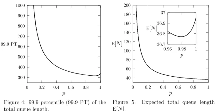
Figures 4 and 5 plot the 99.9 percentile (99.9 PT) and expected value E[N] of the total queue length, respectively, as functions of p. From these figures, we observe the followings. As p goes to zero, both 99.9 PT and E[N] rapidly increase. This phenomenon is due to the fact that once the on-off process is in a long off-period, long off-periods and short on-periods are likely to repeat alternately, and during those intervals, many customers are accumulated in the system. As p becomes large, however, this effect is weakened, and finally, both 99.9 PT and E[N] take their minimums and turn to increase. This implies that there exists some factor to make the queue length increase with p. In what follows, we examine this phenomenon more closely.
300 400 500 600 700 800 900 1000 0 0.2 0.4 0.6 0.8 1 99.9 PT p
Figure 4: 99.9 percentile (99.9 PT) of the total queue length.
40 60 80 100 120 140 160 180 200 0 0.2 0.4 0.6 0.8 1 E[N] p
Figure 5: Expected total queue length E[N]. 36.7 36.8 36.9 37 0.96 0.98 1 E[N] p
Let Ψshort−on, Ψlong−on, Ψshort−off and Ψlong−off denote the events that the on-off process
is in a short on-period, long on-period, short off-period and long off-period, respectively. Figures 6 and 7 plot the conditional expected total queue lengths given those events as functions of p. From Figure 6, we observe that as expected, E[N | Ψlong−off] is always larger
than E[N | Ψshort−off], so that the total queue length in an on-period following a long
of the value of p. Note here that as p goes to one, the contribution of the total queue length in an on-period following a long off-period to E[N | Ψlong−on] becomes large, and we
conjecture that this factor makes E[N | Ψlong−on] increase in the region where p is close to
one, as shown in Figure 7. Moreover, once E[N | Ψlong−on] turns to increase, this affects the
total queue length in the following off-period, and as p goes to one, off-periods following long on-periods are likely to be long off-periods. Thus E[N | Ψlong−off] turns to increase
after E[N | Ψlong−on] does, as shown in Figures 6 and 7.
0 50 100 150 200 0 0.2 0.4 0.6 0.8 1 p E[N | Ψlong−off] E[N | Ψshort−off]
Figure 6: Conditional expected total queue length. 0 50 100 150 200 0 0.2 0.4 0.6 0.8 1 p E[N | Ψlong−on] E[N | Ψshort−on]
Figure 7: Conditional expected total queue length.
Note here that in this particular example,
Pr(Ψlong−on) = Pr(Ψlong−off) = 0.4, Pr(Ψshort−on) = Pr(Ψshort−off) = 0.1.
Therefore the contributions of E[N | Ψlong−on] and E[N | Ψlong−off] to E[N] are four times
as large as those of E[N | Ψshort−on] and E[N | Ψshort−off]. As a result, E[N] increases for p
near one. A similar observation can be applied to the 99.9 percentile, too. 5.4. Impact of correlation between on-off and arrival processes
Finally, we examine the impact of the correlation between on-off and arrival processes on the total queue length N. We consider the following three models, where service times of each class follow the same distribution as in Case GD of subsection 5.1.
In Model 1, the on-off and arrival processes have a correlation, and they are represented by C = " −0.125 − α α α −0.125 − α # , D1(1) = " 0.125 0 0 0 # , D2(1) = " 0 0 0 0.125 # ,
and Dk(n) = O (k = 1, 2) for n = 2, 3, . . ., where Mon = Moff = 1. In Model 2, the on-off
and arrival processes are mutually independent. As for the arrival process, we set a = α,
λ = 0.125 and g = 1 in (5.1) and (5.2). The on-off process is the same as that in subsection
5.1. In Model 3, the on-off and arrival processes have a correlation, and they are represented by C = " −0.125 − α α α −0.125 − α # , D1(1) = " 0 0 0 0.125 # , D2(1) = " 0.125 0 0 0 # ,
and Dk(n) = O (k = 1, 2) for n = 2, 3, . . ., where Mon = Moff = 1. Note here that the
marginal on-off processes in the three models are identical, and so are the marginal arrival processes.
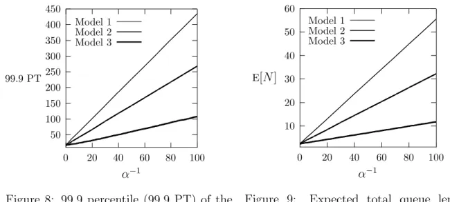
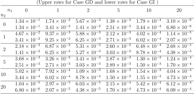
Figures 8 and 9 show the 99.9 percentile (99.9 PT) and expected value E[N] of the total queue length, respectively, as functions of α−1. Note here that as α−1 goes to zero, all the
three models get close to a work-conserving single-server queue, where the arrival process follows a Poisson process with rate 0.125, and service times are i.i.d. and take 2 or 10 with equal probability. This is a reason why both 99.9 PTs and E[N]’s in all the three models converge the same values, respectively, as α−1 → 0. We also observe that 99.9PT and E[N]
in Model 1 (resp. Model 3) are always larger (resp. smaller) than those in Model 2. This is due to the fact the amount of work brought into the system during off-periods in Model 1 (resp. Model 3) is likely to be larger (resp. smaller) than that in Model 2.
50 100 150 200 250 300 350 400 450 0 20 40 60 80 100 99.9 PT α−1 Model 1 Model 2 Model 3
Figure 8: 99.9 percentile (99.9 PT) of the total queue length.
10 20 30 40 50 60 0 20 40 60 80 100 E[N] α−1 Model 1 Model 2 Model 3
Figure 9: Expected total queue length E[N].
A. Proof of Lemma 4.2
From the definition (4.12) of Fm(n), (4.13) is clearly satisfied. (4.14) is proved in the
following way. Let Noff(n) denote an Moff × Moff matrix satisfying
X n∈Z zn1 1 · · · znKK Noff(n) = −Coff− X k∈K D∗ k,off(zk) −1 . (A.1)
From (3.3), (4.12) and (A.1), we have for m = 1, 2, . . .,
X n∈Z zn1 1 · · · znKK Fm(n) = X n∈Z zn1 1 · · · zKnKFm−1(n) · I + θ−1 on Con + X k∈K ∞ X nk=1 zknkDk,on(nk) + Eon,off X n∈Z zn1
1 · · · zKnKNoff(n)Eoff,on
= X n∈Z zn1 1 · · · zKnKFm−1(n)(I + θ−1onCon)
+ X n∈Z zn1 1 · · · znKK θ−1on X k∈K nk X lk=1 Fm−1(n − lkek)Dk,on(lk) + X n∈Z zn1 1 · · · znKK θ−1on X 0≤l≤n
Fm−1(n − l)Eon,offNoff(l)Eoff,on.
Comparing coefficient matrices of zn1
1 · · · zKnK on both sides of the above equation, we obtain
(4.14). Next, we show (4.15) and (4.16). From (3.3) and (A.1), we have
X n∈Z zn1 1 · · · znKK Noff(n) −Coff −X k∈K ∞ X nk=1 zknkDk,off(nk) = I.
Comparing coefficient matrices of zn1
1 · · · znKK on both sides of the above equation yields
Noff(0) (−Coff) = I, Noff(n) (−Coff) − X k∈K nk X lk=1 Noff(n − lkek)Dk,off(lk) = O,
from which (4.15) and (4.16) follow. B. Proof of Theorem 4.6
Post-multiplying both sides of (3.2) by −Coff − D∗off(s) and substituting θon − θonz for s,
we obtain ∞ X m=0 zmv(m)off (θon) " −Coff− ∞ X m=0 zmD(m)off (θon) # = ∞ X m=0 zmv(m)on (θon)Eon,off πonEon,offe 1 Ioff , (B.1) where we use (4.18) and (4.20). Comparing coefficient vectors of zm (m = 0, 1, . . .) on both
sides of (B.1) yields v(0)off(θon) h −Coff − D(0)off(θon) i = v (0) on(θon)Eon,off πonEon,offe 1 Ioff , and for m = 1, 2, . . ., v(m)off (θon) h −Coff − D(0)off(θon) i − m−1X l=0 v(l)off(θon)D(m−l)off (θon) = v(m) on (θon)Eon,off πonEon,offe 1 Ioff .
(4.21) and (4.22) follow the above two equations. C. Total Queue Length Distribution
This appendix summarizes the recursions for the total queue length distribution. Because they are readily derived from the results in Section 4, we omit the proofs.
We first define p(T)(n) (n = 0, 1, . . .) and q(T)
k (n) (k ∈ K, n = 0, 1, . . .) as the
station-ary total queue length distributions at a random point in time and at immediately after departures of class k, respectively.
p(T)(n) = X n∈Z |n|=n p(n), q(T)k (n) = X n∈Z |n|=n qk(n),
Corollary C.1 The p(T)(n) is recursively determined in the following way: p(T)(0) = X k∈K λkq(T)k (0)(−C)−1, and for n = 1, 2, . . ., p(T)(n) = X k∈K " λk ³ q(T)k (n) − q(T)k (n − 1)´+ n X m=1 p(T)(n − m)D k(m) # (−C)−1.
In what follows, we show recursions to compute the q(T)k (n). For this purpose, we introduce the following notations: For k ∈ K, ξ = on, off, n = 0, 1, . . . and m = 0, 1, . . .,
q(T)k,ξ(n) = X n∈Z |n|=n qk,ξ(n), Γ(T)k,ξ(n) = X n∈Z |n|=n Γk,ξ(n), A(T)k,ξ(n) = X n∈Z |n|=n Ak,ξ(n), v(T)k,ξ(n) = X n∈Z |n|=n vk,ξ(n), F(T)m (n) = X n∈Z |n|=n Fm(n).
From Theorem 4.3, we have the following corollary.
Corollary C.2 Under Assumption 4.1, the q(T)k (n) (k ∈ K, n = 0, 1, . . .) is given by
q(T)k (n) =
Ã
ronλk,on
λk
q(T)k,on(n) + roffλk,off
λk
q(T)k,off(n), 0, . . . , 0
!
, where the q(T)k,ξ(n) (k ∈ K, ξ = on, off, n = 0, 1, . . .) is given by
q(T)k,ξ(n) = 1 λk,ξ X m1+m2+m3 +m4=n v(T)k,ξ(m1)[αk,ξ⊗Ak,ξ(T)(m2)]Γ(T)k,ξ(m3) hn Pm4 k,ξ(I − Pk,ξ)e o ⊗ I(Mon) i , if λk,ξ > 0, and otherwise q(T)k,ξ(n) = 0.
As for the Γ(T)k,ξ(n), the following corollary can be obtained from Lemma 4.1.
Corollary C.3 The Γ(T)k,ξ(n) (k ∈ K, ξ = on, off, n = 0, 1, . . .) is determined by the
follow-ing recursion: Γ(T)k,ξ(0) = hI − Pk,ξ⊗ A(T)k,ξ(0) i−1 , Γ(T)k,ξ(n) = n X l=1 Γ(T)k,ξ(n − l)hPk,ξ⊗ A(T)k,ξ(l) i Γ(T)k,ξ(0), n = 1, 2, . . . .
As for the A(T)k,ξ(n), the following recursions can be obtained from Lemma 4.2 and The-orem 4.4.
Corollary C.4 The A(T)k,ξ(n) is given by
A(T)k,ξ(n) =
∞
X
m=0
where the F(T) m (n) is recursively determined by F(T)0 (n) = ( I, if n = 0, O, otherwise, and for m = 1, 2, . . . , F(T)m (n) = F(T)m−1(n)(I + θ−1 onCon) + θon−1 n X l=1 F(T)m−1(n − l)X k∈K Dk,on(l) + θ−1 on " n X l=0
F(T)m−1(n − l)Eon,offN(T)off(l)
#
Eoff,on, n = 0, 1, . . . , with the N(T)off (n), which is given by the following recursion:
N(T)off (0) = (−Coff)−1, N(T)off (n) = Xn l=1 N(T)off (n − l)X k∈K Dk,off(l) N(T)off (0), n = 1, 2, . . . .
Finally, from Theorem 4.5, we obtain the following result.
Corollary C.5 The v(T)k,on(n) (k ∈ K) and the v(T)k,off(n) (k ∈ K) are determined by
v(T)k,on(n) = ∞ X m=0 v(m)on (θon)Dk,onF(T)m (n), n = 0, 1, . . . , v(T)k,off(n) = ∞ X m=0 v(m)off (θon)Dk,off n X l=0
N(T)off (n − l)Eoff,onF(T)m (l), n = 0, 1, . . . ,
respectively.
Acknowledgement
The research of the second author was supported in part by Grant-in-Aid for Scientific Research (C) of Japan Society for the Promotion of Science under Grant No. 15560328. References
[1] A. Federgruen and L. Green: Queueing systems with service interruptions. Operations
Research, 34 (1986) 752–768.
[2] A. Federgruen and L. Green: Queueing systems with service interruptions II. Naval
Research Logistics, 35 (1988) 345–358.
[3] Q.-M. He: Queues with marked customers. Advances in Applied Probability, 28 (1996) 567–587.
[4] Q.-M. He: The versatility of MMAP[K] and the MMAP[K]/G[K]/1 queue. Queueing
Systems, 38 (2001) 397–418.
[5] D. M. Lucantoni, K. S. Meier-Hellstern and M. F. Neuts: A single-server queue with server vacations and a class of non-renewal arrival processes. Advances in Applied
Prob-ability, 22 (1990) 676–705.
[6] D. M. Lucantoni: New results on the single server queue with a batch Markovian arrival process. Stochastic Models, 7 (1991) 1–46.
[7] H. Masuyama and T. Takine: Analysis and computation of the joint queue length dis-tribution in a FIFO single-server queue with multiple batch Markovian arrival streams.
Stochastic Models, 19 (2003) 349–381.
[8] M. F. Neuts: Structured Stochastic Matrices of M/G/1 Type and Their Applications (Marcel Dekker, New York, 1989).
[9] B. Sengupta: A queue with service interruptions in an alternating random environment.
Operations Research, 38 (1990) 308–318.
[10] T. Takine and T. Hasegawa: The workload in the MAP/G/1 queue with state-dependent services: its application to a queue with preemptive resume priority.
Stochas-tic Models, 10 (1994) 183–204.
[11] T. Takine, Y. Matsumoto, T. Suda and T. Hasegawa: Mean waiting times in nonpre-emptive priority queues with Markovian arrival and i.i.d. service processes. Performance
Evaluation, 20 (1994) 131–149.
[12] T. Takine and B. Sengupta: A single server queue with service interruptions. Queueing
Systems, 26 (1997) 285-300.
[13] T. Takine: A recent progress in algorithmic analysis of FIFO queues with Markovian arrival streams. Journal of the Korean Mathematical Society, 38 (2001) 807–842. [14] T. Takine: Distributional form of Little’s law for FIFO queues with multiple Markovian
arrival streams and its application to queues with vacations. Queueing Systems, 37 (2001) 31–63.
[15] T. Takine: Queue length distribution in a FIFO single-server queue with multiple arrival streams having different service time distributions. Queueing Systems, 39 (2001) 349– 375.
Hiroyuki Masuyama
Graduate School of Informatics Kyoto University
Yoshida-honmachi, Sakyo-ku Kyoto 606-8501, JAPAN
![Figure 1 plots the expected total queue lengths E[N ] in Cases GD and GI as functions of α −1](https://thumb-ap.123doks.com/thumbv2/123deta/5787579.1527786/15.892.248.587.254.571/figure-plots-expected-total-queue-lengths-cases-functions.webp)
![Figure 6: Conditional expected total queue length. 0 50100150200 0 0.2 0.4 0.6 0.8 1pE[N|Ψlong−on]E[N|Ψshort−on]](https://thumb-ap.123doks.com/thumbv2/123deta/5787579.1527786/18.892.507.788.282.571/figure-conditional-expected-total-queue-length-ψlong-ψshort.webp)