The Relationship Between Oil Price Shocks and
Macroeconomic Aggregates
著者
Tian Hongzhi
内容記述
学位記番号:論経第73号, 指導教員:村澤康友
Osaka Prefecture University
Graduate School of Economics
The Relationship Between Oil Price
Shocks and Macroeconomic Aggregates
by
Hongzhi Tian
Thesis for the Degree of Doctor of Economics
Abstract
In 1973 and 1979, two oil crises occurred in the international market for crude oil. These oil crises had significant effects on oil-importing countries. Oil is the most important nat-ural energy resource. It is not only a necessary factor in economic development, but is also a strategic material for the safety of a country. Thus, studying the relationship between oil price shocks and economic activity is an important subject in empirical literature. In general, two themes are explored with regard to this subject, namely, the effects of oil price shocks on real economic activity and the factors contributing to oil price changes.
Oil price shocks almost always impose negative effects on real economic activity. These negative effects include inflation, recession, and high unemployment. A recent finding showed that these effects are significantly weaker after 2000 than in the 1970s and 1980s. Thus, economists attempt to clarify the transmission mechanisms of oil price shocks in the economic system and to recommend appropriate monetary policies to reduce such effects.
In Chapters 2 and 3, a Dynamic Stochastic General Equilibrium model and a structural Vector Autoregression model are respectively constructed to confirm the effects of oil price shocks on the Japanese economy.
Chapter 2 discusses an economic system where there are two types of firms in the economy: one type produces intermediate goods and the other produces unique final good. Each intermediate good is produced with capital, labour, and crude oil. The unique final good is produced only by intermediate goods. The primary findings of this chapter are the substitution effects between capital, labour, and oil. We also determine two important changes that have emerged in the last two oil price shocks after the 1980s, that is, the quantity and volatility of oil price shocks have changed across periods.
In Chapter 3, according to the variables in the Vector Autoregression model, the effects of oil price shocks on the Japanese economy are analysed using four steps. Step 1 merely
analyses the relationship between oil price shocks and real GDP. To explain the results in Step 1, five macroeconomic aggregates in the expenditure side of national income (private consumption, total investment, government expenditure, exports, and imports) must be enumerated in detail first. This detailed enumeration is performed in Step 2. In Step 3, the export and production of automobiles in the Japanese economy, which are affected by oil price shocks, are tackled in more detail. Finally, in Step 4, we explain all the responses of the Japanese economy through the weights of each term in the expenditure side of national income. A feature of the Japanese economy is that, after the 1980s, the weights of private consumption and total investment have decreased, whereas the weights of expenditure of government, exports, and imports have all increased. This approach can also explain why the effects of oil price shocks are weaker after 2000 compared with those in the 1970s and 1980s. The Granger causality between Japan’s total investment and exports after 1985 is also explained further. The main finding of this paper is that the scale of effects of oil price shocks in one country relates to the economic structure of that country.
On the other hand, a common viewpoint about the causes of oil price changes that has emerged recently is that the shortage in supply from the international market results in the increase of real oil price. Moreover, crude oil production was easily affected by the war and political strife in the Middle East before the 2000s. However, since 2002, no observable reduction has occurred in crude oil production, despite the increase in real oil prices. During the same period, the remarkable, rapid economic growth of China, which entailed high levels of oil consumption, became associated with the international crude oil market. Thus, we pay close attention to the role of China’s real economic activity in the increase of real oil prices.
Chapter 4 aims to confirm whether the Chinese economy indeed affected real oil prices in recent decades. To determine this effect, a structural Vector Autoregression model is used. The shocks of oil market-specific and OECD demands are found to have consid-erably affected the real price of crude oil from 1994 to 2010. In addition, prior to 2002, China’s real economic activity did not have sufficient power to affect real oil prices. Since 2002, however, the demand shocks of China’s economic activity positively affected world oil price, but this effect was only temporary and minimal. Until 2010, China’s oil con-sumption accounted for a very small portion of total world concon-sumption, which possibly
explains its minimal effect on real oil prices. As an important application of the structural Vector Autoregression model, we plot the cumulative contributions of each shock to real oil prices in two subsample periods.
Contents
Abstract i
List of Figures vi
List of Tables vii
Acknowledgements viii
1 Introduction 1
2 Effects of Oil Price Shocks on Japan’s Economy: A DSGE Approach 4
2.1 Introduction . . . 4
2.2 Oil Price Shocks and VAR model . . . 6
2.2.1 Oil Price Shocks . . . 6
2.2.2 VAR Model . . . 7 2.3 Model . . . 10 2.3.1 Household . . . 10 2.3.2 Final Good . . . 11 2.3.3 Intermediate Goods . . . 11 2.3.4 Market Equilibrium . . . 13
2.3.5 Oil Price Shocks . . . 13
2.4 The Steady State of System . . . 14
2.5 Simulation . . . 14
2.6 Conclusions . . . 16
3 The Effects of Oil Price Shocks on the Japanese Economy 19 3.1 Introduction . . . 19
3.2 Model Specification . . . 21
3.2.1 Oil Price in the Japan Case . . . 21
3.2.2 Oil Price Shocks . . . 23
3.2.3 Exogeneity of Oil Price . . . 24
3.3 Model . . . 25
3.3.1 Structural Break Point . . . 25
3.3.2 Unit Root Tests of Variables . . . 25
3.3.3 Structural Bivariate VAR Model . . . 25
3.3.4 Empirical Results . . . 29
3.4 Two Frameworks of Economic Theory . . . 34
3.5 Conclusions . . . 35
4 The Role of China’s Real Economic Activity in Oil Price Changes 38 4.1 Introduction . . . 38
4.2 Literature Review . . . 39
4.3 Model Specification . . . 41
4.3.1 Sample Period . . . 41
4.3.2 Variables and Data . . . 41
4.4 Structural VAR Model . . . 42
4.4.1 Model . . . 42
4.4.2 Identifying Restrictions . . . 44
4.5 Empirical Results and Analyses . . . 45
4.5.1 Impulse Response Functions . . . 45
4.5.2 Four Types Shocks . . . 48
4.5.3 Historical Decomposition of the Real Price of Oil . . . 50
4.5.4 Share of China’s Oil Consumption in World Total Consumption . 50 4.6 Conclusions . . . 53
List of Figures
2.1 Oil Price . . . 7 2.2 Real GDP . . . 8 2.3 Real Wage . . . 8 2.4 CPI . . . 9 2.5 Employment . . . 92.6 The Results of Simulation . . . 16
3.1 Three types of oil prices . . . 22
3.2 WTI price and real oil price for Japan’s economy . . . 23
3.3 IRFs of Real GDP to oil price shocks . . . 29
3.4 IRFs of expenditure side of national income to oil price shocks . . . 29
3.5 IRFs of export and production of automobile to oil price shocks . . . 30
3.6 The growth rate of total investment and export before 1986 . . . 32
3.7 The growth rate of total investment and export after 1986 . . . 32
3.8 The growth rate of oil price . . . 35
4.1 Real oil price of WTI and RAC . . . 43
4.2 IRFs to one standard deviation structural shocks of 1994-2010 . . . 46
4.3 IRFs to one standard deviation structural shocks of 1994-2001 . . . 46
4.4 IRFs to one standard deviation structural shocks of 2002-2010 . . . 47
4.5 Four types of the structural shocks 1995-2001 . . . 49
4.6 Four types of the structural shocks 2003-2010 . . . 49
4.7 Historical decomposition of real price of oil for 1994-2001 . . . 51
4.8 Historical decomposition of real price of oil for 2002-2010 . . . 51
List of Tables
2.1 Increase Rate of Oil Price in Each Quarter . . . 6
2.2 The Value of Parameters . . . 15
3.1 Granger causality test the oil price and production from 1975 to 2010 . . 24
3.2 Granger causality test the oil price and Japan’s real GDP . . . 24
3.3 Unit root tests . . . 26
3.4 The optimal lags length of each model . . . 28
3.5 The one standard deviation of oil price in each model . . . 28
3.6 Granger causality test total investment and exports from 1973 to 1985 . . 33
3.7 Granger causality test total investment and exports from 1986 to 2010 . . 33
Acknowledgements
I acknowledge the guidance, supports and direction of Professor Yasutomo Murasawa from College of Economics, Osaka Prefecture University who oversees this research.
I also would like to acknowledge Professor Shigeru Matsukawa from the same college, who brought me into the economics world.
In addition, the author also would like to acknowledge helpful comments and sugges-tions on this thesis from all staffs in the same college.
At last, I am very grateful to Japanese government for Monbukagakusho (MEXT) Scholar subsidizing my studies.
Chapter 1
Introduction
In 1973 and 1979, two oil crises occurred in the international market for crude oil. These oil crises had significant effects on oil-importing countries. Oil is the most important nat-ural energy resource. It is not only a necessary factor in economic development, but is also a strategic material for the safety of a country. Thus, studying the relationship between oil price shocks and economic activity is an important subject in empirical literature. In general, two themes are explored with regard to this subject, namely, the effects of oil price shocks on real economic activity and the factors contributing to oil price changes.
Oil price shocks almost always impose negative effects on real economic activity. These negative effects include inflation, recession, and high unemployment. A recent finding showed that these effects are significantly weaker after 2000 than in the 1970s and 1980s. Thus, economists attempt to clarify the transmission mechanisms of oil price shocks in the economic system and to recommend appropriate monetary policies to reduce such effects.
In Chapters 2 and 3, a Dynamic Stochastic General Equilibrium model and a structural Vector Autoregression model are respectively constructed to confirm the effects of oil price shocks on the Japanese economy.
Chapter 2 discusses an economic system where there are two types of firms in the economy: one type produces intermediate goods and the other produces unique final good. Each intermediate good is produced with capital, labour, and crude oil. The unique final good is produced only by intermediate goods. The primary findings of this chapter are the substitution effects between capital, labour, and oil. We also determine two important
changes that have emerged in the last two oil price shocks after the 1980s, that is, the quantity and volatility of oil price shocks have changed across periods.
In Chapter 3, according to the variables in the Vector Autoregression model, the effects of oil price shocks on the Japanese economy are analysed using four steps. Step 1 merely analyses the relationship between oil price shocks and real GDP. To explain the results in Step 1, five macroeconomic aggregates in the expenditure side of national income (private consumption, total investment, government expenditure, exports, and imports) must be enumerated in detail first. This detailed enumeration is performed in Step 2. In Step 3, the export and production of automobiles in the Japanese economy, which are affected by oil price shocks, are tackled in more detail. Finally, in Step 4, we explain all the responses of the Japanese economy through the weights of each term in the expenditure side of national income. A feature of the Japanese economy is that, after the 1980s, the weights of private consumption and total investment have decreased, whereas the weights of expenditure of government, exports, and imports have all increased. This approach can also explain why the effects of oil price shocks are weaker after 2000 compared with those in the 1970s and 1980s. The Granger causality between Japan’s total investment and exports after 1985 is also explained further. The main finding of this paper is that the scale of effects of oil price shocks in one country relates to the economic structure of that country.
On the other hand, a common viewpoint about the causes of oil price changes that has emerged recently is that the shortage in supply from the international market results in the increase of real oil price. Moreover, crude oil production was easily affected by the war and political strife in the Middle East before the 2000s. However, since 2002, no observable reduction has occurred in crude oil production, despite the increase in real oil prices. During the same period, the remarkable, rapid economic growth of China, which entailed high levels of oil consumption, became associated with the international crude oil market. Thus, we pay close attention to the role of China’s real economic activity in the increase of real oil prices.
Chapter 4 aims to confirm whether the Chinese economy indeed affected real oil prices in recent decades. To determine this effect, a structural Vector Autoregression model is used. The shocks of oil market-specific and OECD demands are found to have consid-erably affected the real price of crude oil from 1994 to 2010. In addition, prior to 2002,
China’s real economic activity did not have sufficient power to affect real oil prices. Since 2002, however, the demand shocks of China’s economic activity positively affected world oil price, but this effect was only temporary and minimal. Until 2010, China’s oil con-sumption accounted for a very small portion of total world concon-sumption, which possibly explains its minimal effect on real oil prices. As an important application of the structural Vector Autoregression model, we plot the cumulative contributions of each shock to real oil prices in two subsample periods.
Chapter 2
Effects of Oil Price Shocks on Japan’s
Economy: A DSGE Approach
2.1
Introduction
Recent empirical studies have revealed that the effects of oil shocks became muted after the mid-1980s. For example, Sanchez (2008) studied oil price shocks and Kilian (2007) examined oil supply shocks in major industrialized countries. Comparing the distinct macroeconomic specification between these countries, they obtained similar conclusions: the typical response to an oil shock is a decrease in the real GDP growth rate and real wage, leading to inflation and so on. This performance is often called stagflation. How-ever, in the study of Blanchard and Gali (2008), Japan deviated from this general response; an increase, instead of a decrease, was the impulse response of the real GDP in Japan to oil price shocks. Blanchard and Gali (2008) could not properly explain this phenomenon. The purpose of this paper is to explain why an increase is the response of Japan’s real GDP to oil price shocks, and to analyze other macroeconomic variables. We ex-plore the features of the two recent oil price shocks. We first use the VAR model to find the actual effects of oil price shocks to macroeconomic aggregate variables, and then build the theoretical model for the sake of a more detailed analysis. We consider oil as a major production factor and construct a dynamic stochastic general equilibrium model (DSGE) focusing on Japan’s economy. This model is similar to the one used by Leduc and Sill (2004) which, in turn, is an extension of the real business cycle model presented in Finn (1995). As such, the model belongs to the New Keynesian tradition in
that forward-looking agents solve dynamic optimum problems with rational expectations in an environment of slow price adjustments.
As far as the oil shocks are concerned, there are two main definitions in empirical analysis: oil supply shocks and oil price shocks. According to Kilian (2007), oil supply shocks are often analyzed as the reason behind an oil crisis; however the statistic data of worldwide oil production is difficult to search. In fact, shortages in oil production may not bring oil shocks, such as during the Persian Gulf War in 1990. This paper adopts oil price shocks as oil shocks with a new method definition. In this method, West Texas Intermediate (WTI) oil price, which is tacitly approved as the international oil price, is used. In our model, oil prices directly use the data of WTI (in US dollars) because Japan’s reliance on oil import is 99.7% (data from OECD: Energy Balances of OECD Countries 2008).
There are also two main methods of investigating the effects of oil price shocks to cer-tain macroeconomic variables: using an input-output table and using a dynamic model. As seen in Fujikawa et al. (2007), the fault of the first method is that only the target vari-able can be analyzed within a matrix and other economic varivari-ables cannot be explained. This paper uses the second method, which applies econometric software to simulate the dynamic processes of all variables, which can easily vary the values of parameters to observe the size of effects of oil price shocks.
The main finding of this paper is that the two recent oil price shocks are different from the previous two occurrences. Based on our definition of oil price shocks, the quantity and volatility of shocks have changed across periods, especially in the last oil price shock; oil prices increased in one quarter and then immediately decreased in the next quarter. This is a very important reason why the effects of oil price shocks have become smaller after the 1980s. Moreover, we apply microeconomic theory to successfully account for why the real GDP in Japan continue to rise when the oil price shocks occur. Oil is a normal good; once its price is rising, its demand should decrease. According to Japanese data, if the demands of two other production factors are increase, real output should also rise.
This paper is organized as follows: in Section 2, we use the VAR model to confirm the effects of oil price shocks; in Section 3, we develop the DSGE model; in Section 4, we compute the steady state of this system; and in Section 5, we calibrate the parameters by software to simulate the dynamics of this model. Section 6 provides our conclusions.
2.2
Oil Price Shocks and VAR model
2.2.1
Oil Price Shocks
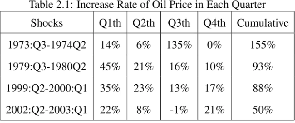
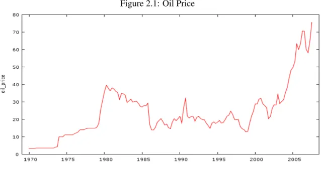
Figure 1 shows the evolution process of oil prices from 1970:Q1 to 2007:Q4. This paper uses the dollar price for Japan directly without considering exchange rates because Japan relies very highly on oil imports and international oil prices are usually expressed by WTI data. We define an oil price shock as the cumulative increase rate of above 50% in the nominal oil price during one year. According this definition, there have been four periods of oil price shock occurrences, namely, 1973:Q3-1974:Q2, 1979:Q3-1980:Q2, 1999:Q2-2000:Q1, and 2002:Q2-2003:Q1. We find that the first two shock occurrences were due to the Yom-Kippur War and the Arab Oil Embargo, with an increase of 135% with a 45%, respectively, in one quarter. This is in contrast to the last two occurrences where oil price shocks rose gradually; although the rates reached 88% and 50%, respectively, the increase spanned four quarters (Table 1). In fact, there was no war in the primary oil-producing areas during these two occurrences. In particular, oil prices continuously increased from 2003 through 2007. The different speed and volatility of increases in oil prices are essential distinctions between the first and last two shock occurrences.
Table 2.1: Increase Rate of Oil Price in Each Quarter
Shocks Q1th Q2th Q3th Q4th Cumulative
1973:Q3-1974Q2 14% 6% 135% 0% 155%
1979:Q3-1980Q2 45% 21% 16% 10% 93%
1999:Q2-2000:Q1 35% 23% 13% 17% 88%
2002:Q2-2003:Q1 22% 8% -1% 21% 50%
Some studies have indicated that the effects of the last two shocks on macroeconomic performance have become smaller than the first two shocks (e.g., Blanchard and Gali, 2008; Kilian, 2007). In Blanchard and Gali’s paper, the reasons the effects of oil price shocks have been recently weakened are the decrease in real wage rigidities, smaller oil share in production, and improvements in monetary policy. For the last two shock occur-rences, this paper uses the microeconomic view, that is, short run and long run. In the
Figure 2.1: Oil Price
short run, when oil prices rise abruptly, firms cannot immediately adjust the quantities of their capital and labour, thus the effects of oil price shocks are large. Oil prices contin-uously increased from 2003 through 2007. In the long run, when oil prices rise slowly, firms can change their capital and labour in order to offset the effects of the shock.
2.2.2
VAR Model
We first utilize the VAR model to provide evidence for Japan’s economy. The VAR model includes five variables: real GDP, CPI, real wage, oil price, and employment. All vari-ables are data cited quarterly in the OECD economic outlook database, analysis period, 1984:Q1-2007:Q4. In the computation method, oil prices are expressed in log differences. Real GDP and employment are expressed in logarithms. Each equation in the VAR model contains four lags for each variable, including a constant term and a quadratic and trend fitted measure of productivity growth. The confidence interval is 95% and the forecast period is 12 quarters. The magnitude of the price shock increase is normalized at 10% of the oil price.
Figures 2 to 5 show the results of the VAR model computation.
Typically, the impulse responses of oil price shocks are decreases in real GDP, em-ployment, and real wage, in addition to high inflation. When oil prices increase, produc-tion costs rise and producproduc-tion output decreases. Accordingly, real wage and employment levels also decrease. However, we note that the impulse responses of Japan to oil price
shocks have a unique style (see Figures 2-5). Real GDP, employment, and real wage in-crease, only CPI inflation fits the typical responses. The size of the four variables affected by oil price shocks is very mild. This point is a unique feature of the Japanese economy.
Figure 2.2: Real GDP
Figure 2.3: Real Wage
As asserted by Blanchard and Gali (2008), Japan is different from other G7 countries, although Gali’s model cannot explain why. To offer an explanation, oil price shocks are modeled in this paper as an unexpected exogenous variable. In the next section, we introduce the DSGE model to analyze this phenomenon.
Figure 2.4: CPI
2.3
Model
The economy includes a large number of identical and infinitely lived households. There are two types of firms in the economy: one type produces intermediate goods and the other produces unique final goods. Each intermediate good is produced with capital, labour, and crude oil. The unique final good is produced only by the intermediate goods, which can be used for consumption and investment.
2.3.1
Household
In period t, each household’s utility function is U (Ct, Ht) =
Ct1−ν 1 − ν −
Ht1+η
1 + η, (3.1)
where Ctis the consumption of the representative household, and Htis the labour supply
of the representative household. Parameters ν and η respectively denotes the risk aversion coefficient of consumption and labour supply. The household’s lifetime expected utility is defined as follows: Et ∞ X s=0 ρsU (Ct+s, Ht+s), (3.2)
where 0<ρ<1 is a subjective discount factor. Et represents rational expectation of the
household for future. In each period, the household faces the budget constraint:
Pt(Ct+ It) + Bt ≤ PtrtKt+ Nt+ Bt−1(1 + Rt−1) + 1
Z
0
Π(i)di, (3.3)
where Ptis the nominal price of the final good in period t, It is the investment, Btis the
bonds, wtis real wage, rtis real rental rate of capital, Ktis the physical capital, Rtis the
nominal interest rate, Πt(i) is the profit of firm i owned by households, and Ntrepresents
transfer from government.
Capital stock is accumulated as follows:
Kt+1= It+ (1 − δ)Kt, (3.4)
where δ ∈ (0, 1) is the depreciation rate of the capital. Maximizing Equation (3.2) subject to Equation (3.3) and Equation (3.4) by using Bellman equation, we obtain the necessary condition for the representative households’ optimization problem:
Ct−ν − e−πt+1ρE
tCt+1−ν(1 + Rt) = 0, (3.6)
Ct−ν− ρEtCt+1−ν(1 − δ + rt+1) = 0. (3.7)
2.3.2
Final Good
Final good is produced with only intermediate goods, according to a technology described by the following CES function:
Yt= ( 1 Z 0 Xt(i)θdi) 1 θ, (3.8)
where θ ∈ (0, 1), and 1−θ1 is elasticity of substitution among intermediate goods Xt(i)
produced by the i-th firm. Ytis the output of final good. The profit function of producing
the final good is defined as:
Πt= PtYt− 1
Z
0
Pt(i)Xt(i)di, (3.9)
where Pt(i) is the price of i-th intermediate good. Differentiating Equation (3.9) with
respect to Xt(i), we can obtain the demand function for i-th intermediate good:
Xt(i) = (
Pt(i)
Pt
)θ−11 Yt. (3.10)
2.3.3
Intermediate Goods
Using three production factors, capital, labour and crude oil, the i-th firm produces an intermediate good with constant returns-to-scale technology. The form of production function is
Xt(i) = Kt(i)αHt(i)βFt(i)1−α−β, (3.11)
where Kt(i), Ht(i) and Ft(i) are the physical capital, labour input and crude oil,
respec-tively, used by the i-th firm in the production process. α, β are capital share and the labour share, respectively. All considerations are founded on the assumption that the production factor markets are perfectly competitive; however, the market of intermediate goods is monopolistically competitive in this economic model. For each firm producing interme-diate good, the profit function is as follows:
where Ct(i) is nominal cost of intermediate good i. It consists of:
Ct(i) = PtrtKt(i) + PtwtHt(i) + Poil,tFt(i), (3.13)
where Poil,tis the nominal price of crude oil in period t. Minimizing the Equation (3.13)
subject to Equation (3.11), we obtain the first-order conditions: rt= λt(i)Et αXt(i) Kt(i) , (3.14) wt= λt(i)Et βXt(i) Ht(i) , (3.15) poil,t= λt(i)Et (1 − α − β)Xt(i) Ft(i) , (3.16)
where poil,tis real oil price. λt(i) is a multiplier lagrangian function, which is equal to the
marginal cost of producing intermediate good i-th firm. More concretely, we have mct(i) = ( rt α) α(wt β ) β( poil,t 1 − α − β) 1−α−β. (3.17)
Let Φt+srepresent the marginal value of one unit of money held in period t+s in terms
of money held in period t.
Φt+s = ρs
Uc(Ct+s)Pt
Uc(Ct)Pt+s
. (3.18)
The firms are under assumed monopolistic competition and produce different inter-mediate goods. In each period, any firm producing an interinter-mediate good is assumed to be able to reset its price with a constant fraction 1 − γ, while the rest, γ, is assumed to keep their prices unchanged. This price-setting rule is the Calvo scheme. It is as follows:
P θ θ−1 t = (1 − γ)(P ∗ t) θ θ−1 + γP θ θ−1 t−1, (3.19)
where Pt∗denotes the optimal price by set at time t. Consider profit maximization problem
for the i-th firm producing intermediate good i: Et
∞
X
s=0
γsΦt+s[Pt∗Xt+s(i) − Ct+s(i)]. (3.20)
The first order condition to Equation (3.20) associated with the firm’s choice of Pt∗ is
the following: Et ∞ X s=0 γsΦt+sXt+s(i)Pt+s[θ Pt∗ Pt+s − mct(i)] = 0. (3.21)
By taking the first order Taylor expansion of Equation (3.21) at the steady state, we obtain the following relation:
ˆ Pt∗ = Et ∞ X s=0 γsρsπt+s+ (1 − γρ)Et ∞ X s=0 γsρsmcˆt+s. (3.22)
By taking the first order Taylor expansion of Equation (3.19), we obtain the following relation: πt= ( 1 − γ γ ) ˆP ∗ t. (3.23)
By combining Equations (3.22) and (3.23), we obtain the inflation rate:
πt= ρEtπt+1+
(1 − γ)(1 − ργ)
γ mcˆt. (3.24)
2.3.4
Market Equilibrium
From the market clearing condition of the final good, we have the following equations:
Yt= Ct+ It, (3.25) Kt= 1 Z 0 Kt(i)di, (3.26) Ht= 1 Z 0 Ht(i)di, (3.27) Ft= 1 Z 0 Ft(i)di. (3.28)
2.3.5
Oil Price Shocks
Based on the oil price of 1984 through 2007, we estimate that the crude oil price follows AR (1) process:
lnpoil,t= 0.993lnpoil,t−1+ εt, εt ∈ N(0, 0.012), (3.29)
2.4
The Steady State of System
The endogenous variables of this system are: Ct,It,Kt,Ht,Ft,poil,t,Yt,mct,πt,rt,wt,and
Rt.The next step is to find necessary equations that describe the equilibrium law of motion
for this system. These equations should include the state Equation (3.4); the first order condition derived either as the Euler Equation (3.6) or from the Bellman Equation (3.5), (3.7), and (3.11), (3.14), (3.15), (3.16), (3.17), (3.24), (3.25); and the oil price shocks Equation (3.29). The steady state of this system satisfies following equations:
I = δK, (4.1) r = αmcY K, (4.2) w = βmcY H, (4.3) poil = (1 − α − β)mc Y F, (4.4) π = ρπ + (1 − γ)(1 − γρ) γ (mc − mc), (4.5) lnpoil = 0.993lnpoil, (4.6) C−νw = µHη, (4.7) Y = KαHβF1−α−β, (4.8) 1 − δ + r = 1 + R, (4.9) Y = C + I, (4.10) ρ = 1 1 + R, (4.11) mc(i) = (r α) α(w β) β( poil 1 − α − β) 1−α−β. (4.12)
2.5
Simulation
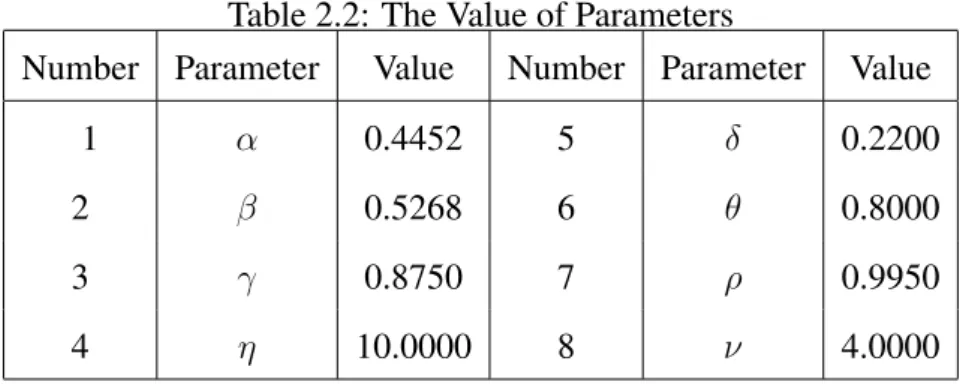
There are 8 parameters in this mode: α, β, γ, η, δ, θ, ρ, ν. Among these parameters, α, η and ν are cited from Ueda (2001). θ is cited by Odani (2002). δ is cited from Otsu (2008). ρ is set at 0.995, in reference to Saitou et al. (2007). γ is cited from Sugo and Ueda (2008). Labour share β is computed from the average value of the proportion of employee compensation to GDP, based on Japanese 1984-2007 data. Oil share is cited from Hirata (2006). The values of parameters are listed in Table 2.
Table 2.2: The Value of Parameters
Number Parameter Value Number Parameter Value
1 α 0.4452 5 δ 0.2200
2 β 0.5268 6 θ 0.8000
3 γ 0.8750 7 ρ 0.9950
4 η 10.0000 8 ν 4.0000
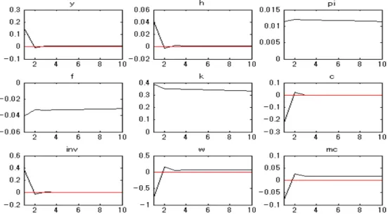
We use the econometrics software, Dynare, which automatically calculates eigenval-ues and carries out the stability analysis. The results of simulation are shown in Figure 6. The horizontal axis represents time, while the vertical axis represents percentage de-viations from the steady state. The time unit is a quarter; the size of oil price shocks is normalized, meaning that the price of crude oil rises at 10% per period. The observation length is 10 quarters. In each figure, the observed endogenous variable is attached to the figure’s name. In this simulation, the value of gamma is set at 0.875, similar to Sugo et al. (2008).
Figure 6-pi depicts the impulse response of inflation rate to oil price shocks. When the price of crude oil is rising at a rate of 10%, the inflation rate is also rising at a rate of 0.1%. Accompanying the increase in oil price is the rising marginal cost of the inter-mediate good, as shown in Equation (3.21). From Equation (3.24), inflation rate depends on the value of gamma and the marginal cost of the intermediate good. This result is also consistent with Figure 4. High price is the typical impulse response of oil price shocks.
Figures 6-h, 6-k, and 6-y present labour demand, capital demand and output. Crude oil is one of the major production factors, as shown in Equation (3.11). Once the crude oil price rises as a result of the substitution effects of production factors, the demand for crude oil decreases; however, the demands for labour and capital increase. Two of the three production factors increase; oil share is small, hence the output increases.
Unfortunately, this DSGE model cannot explain the impulse response of real wage to oil price shocks (see Figure 6-w). The real wage declined in our simulation. Yet in Section 2, we have shown that real wage increases when there is an oil price shock (see Figure 3 with VAR model). This result is similar to typical conclusions, for example, Kilian’s (2007) conclusion. Our model is under sticky prices and flexible wages. Using
the results of Blanchard and Gali (2007), who studied the New Keynesian model with both sticky prices and wages, may explain this problem in future.
Figure 2.6: The Results of Simulation
2.6
Conclusions
For the first time, this paper uses the DSGE model to analyze the impact of the crude oil price shocks to the Japanese inflation rate, and simulates the dynamics of this model using the software, Dynare. We can conveniently change the values of parameters to observe the dynamic behavior of economic variables. In addition, with this model, we can also observe the dynamic behavior of macroeconomic variables such as investment and consumption, among others.
Given the model, this paper successfully explains why real GDP increases even when there is crude oil price shock. For the first time, the relations of the substitution effects of the production factors are shown.
The main finding of this paper is that inflation rate influenced by crude oil price shocks is rather negligible in Japan. In 2007, the crude oil price shocks did not bring panic to Japan, and commodity prices even became stable.
While this study ignores sticky wages and the technological improvements in the pro-duction functions, these results may be useful in explaining why real wage increases in our given model.
Data Sources
Items Sources
WTI EIA
OPEC basket price EIA
Brent spot price EIA
Emplpyee compensation of Japan’s labor OECD’s Economic Outlook Database
Japan’s GDP OECD’s Economic Outlook Database
Note: EIA is the Energy Information Administration. Appendix
The code of DSGE model in Dynare: var c w h R pi rental y k f mc p o inv ; varexo e o ;
parameters v eta theta sigma rho gamma delta rho i alpha beta rho o ; v=4; eta=10; theta=0.8; rho=0.995; gamma=0.875; delta=0.022; alpha = 0.445; beta= 0.5268; rho o =0.975; model (linear); k=inv+(1-delta)*k(-1);
y=k(-1)ˆ alpha*hˆ beta*fˆ (1-alpha-beta); rental=mc*alpha*y/(k(-1));
w=mc*beta*y/h;
p o=mc*(1-alpha-beta)*y/f;
pi=rho*pi(+1)+(ln(mc)-ln(5.13))*(1-gamma)*(1-rho*gamma)/gamma; ln(p o)=0.993*ln(p o(-1))+0.0+e o;
mc=(rental/alpha)ˆalpha*(w/beta)ˆbeta*(p o/(1-alpha-beta))ˆ(1-alpha-beta); w*cˆ(-4)=hˆ10; cˆ(-4)=rho*(c(+1))ˆ(-4)*2.718ˆ(-pi(+1))*(1+R); 1-delta+rental(+1)=(1+R)*2.718ˆ(-pi(+1)); y=c+inv; end; initval; c=2.384; w=45.998; h=1.036; R=0.005; pi=0; rental=0.027; y=2.97; k=26.64; f=0.1865; mc=5.129; p o=1; inv=0.586; end; shocks; var e o=0.1ˆ2; end; check;
Chapter 3
The Effects of Oil Price Shocks on the
Japanese Economy
3.1
Introduction
After the first and second global oil crises in the 1970s, empirical studies on the effects of oil price shocks on macroeconomic aggregates have been published. A widely accepted consensus in empirical literature is that oil price shocks generally cause inflation and de-crease real GDP and real wage for oil-importing countries. Hamilton (1983) uses US data from 1948 to 1980 to investigate the significant relationship between oil price changes and real GNP growth, and reports an inverse correlation between oil price fluctuations and economic performance. Other researchers, particularly Kilian (2008a, b) who uses a vector autoregession (VAR) model and Hamilton (2003) who uses a nonlinear model, have obtained similar results for the US case.
Using periods to distinguish the effects of oil price shocks, Blanchard and Gali (2007) find that oil price shocks after 1985 have a less severe effect on most industrialized coun-tries economy than on those before 1985 because of the changes in economic structure (e.g., use of less petroleum products in production, more flexible labour markets, and improved monetary policy).
Using countries to distinguish the effects of oil price shocks, some empirical literature focusing on the Organisation for Economic Cooperation and Development (OECD) or France, Germany, Italy, Japan, United Kingdom, United States, and Canada (G7) indicate that unlike the results found in most industrialized countries, those in the context of the
Japanese economy vary across different models. Kilian (2008a) and Cologno and Manera (2008) demonstrate that oil price shocks did not significantly affect Japan’s real GDP growth in the 1970s and 1990s. Lee et al. (2001) observe a negative cumulative effect of oil price shocks on Japan’s real GDP from 1960 to 1996 (In fact, this negative relationship is infinitesimal). Alternatively, Blanchard and Gali (2007) and Jimenez-Rodriguez and Sanchez (2005) use different structural VAR models to confirm the positive relationship between oil price shocks and Japan’s GDP growth from 1985 to 2007 and 1972 to 2001. No study has been conducted explaining Japan’s unusual reaction to oil price shocks. Explaining these conflicting results remains a challenge.
As the effects of oil price shocks according to history and region show different results, as an empirical study, we should appoint a specific period and country. Japan is a net oil-importing country, and it has no domestic oil-mining sector. Nevertheless, it has a strong automobile sector. These features of the Japanese economy may show different responses to oil price shocks. Thus, this paper investigates the effects of oil price shocks on the Japanese economy, whether they relate to its economic structure in the period of 1973-2010. In the so-called economic structure, we focus on each term in the expenditure side of Japan’s national income (i.e., private consumption, total investment, government expenditure, exports, and imports) and observe their responses to oil price shocks using the structure bivariate VAR model.
Our main finding is that oil price shocks affected Japan’s economy in two sub-periods. (1) In the period of 1973-1985, similar to other oil-importing countries, Japan’s economy showed a typical response to oil price shocks: decrease in real GDP. (2) In the period of 1986-2010, oil price shocks did not significantly affect Japan’s real GDP growth. Specifi-cally, there were not only negative but also positive effects of oil price shocks on some sec-tors. For example, automobile exports increased with oil price shocks. These responses considerably differ from those of the US economy (Hamilton, 2009b). Automobile ex-ports account for the bulk of Japanese exex-ports (based on the trade statistics of Japan), and this positive contribution is an important feature of Japan’s economy. Although private consumption has the largest share in the expenditure side of Japan’s national income, it has not exhibited a significant response to oil price shocks in the past two decades. We also find the positive responses of total investment after 1985. Moreover, we discover
the Granger causality between total investment and export in Japan’s economy, which is slightly surprising. We provide some theories to support our results.
The remainder of this paper is organized as follows. Section 3.2 clarifies some basic problems about oil price shocks. Section 3.3 develops the research model and method-ology, and presents our analysis of the oil price shock responses. Section 3.4 introduces partial and general equilibrium analyses with economic theory to explain the phenomenon of total investment increase in oil price shocks. Section 3.5 concludes this paper.
3.2
Model Specification
3.2.1
Oil Price in the Japan Case
Three main types of nominal oil price statistics (US dollar per barrel) exist in the interna-tional oil market:
(1) Organization of Petroleum Exporting Countries (OPEC) basket price: Since 1987, OPEC countries have managed crude oil production and adjusted oil prices accordingly by simply averaging the basket prices of the seven main crude oil-producing fields. However, this price does not have a significant influence on the international crude oil market.
(2) Brent spot price: About two-thirds of the international crude oil supply is priced relative to the Brent spot price, which combines the prices of 15 different oil-producing fields in the Brent and Ninian areas of the North Sea.
(3) West Texas Intermediate (WTI): This statistics is the most important US bench-mark. It has the longest quarterly records dating back to 1946. WTI price is commonly used in empirical studies.
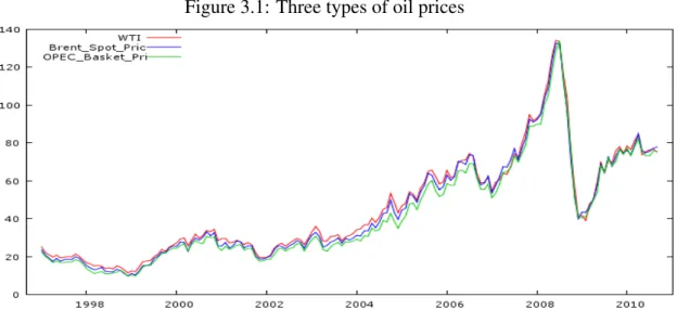
Since 2005, about 90% of Japanese oil imports have come from the Middle East (based on the trade statistics of Japan). Hence, the OPEC basket price should be used. However, no available data can be found prior to 1987, and monthly data are only avail-able beginning 1997. Generally, the OPEC benchmark is preferred for as long as the series data on oil prices are available. Moreover, using the OPEC data series from 1997 to 2010 enables the comparison with other oil price benchmarks (Figure 3.1). Moreover, compar-ative data nearly correspond to historical data. WTI prices are always the highest, whereas
OPEC basket prices are consistently the lowest. In this study, the WTI benchmark is used because it has the most extensive data available.
Figure 3.1: Three types of oil prices
Most empirical literature utilizes unadjusted nominal WTI price (Blanchard and Gali, 2007) or real WTI oil price, which is computed by dividing the nominal price by the US CPI (Jimenez-Rodriguez and Sanchez, 2005), even when the home currency of the country under study is not US dollars. For the Japanese economy, the US CPI is not an important index. Moreover, these oil price indices can provide results but not reflect the real effects of oil price shocks on non-dollar countries. Japan is a net oil-importing coun-try; hence, the influence of exchange rates on oil imports, particularly the yen-US dollar exchange rates that are easily affected by global economic events, must be considered.
In this study, WTI price is multiplied by the yen-US dollar exchange rate (to obtain the nominal price of the Japanese yen) and is then divided by Japan’s CPI (to obtain the real oil price). Exchange rate fluctuations can either magnify or reduce the size of oil price shocks for the Japanese economy, particularly for its oil importation. The 1985 Plaza Ac-cord significantly affected the Japanese yen exchange rate. Figure 3.2 shows that, before 1985, yen depreciation magnified the size of oil price shocks, thereby adversely affect-ing the Japanese economy in 1973 and 1979. Exchange rate fluctuations also affected the Japanese economy during the oil price shocks. After 1985, real oil prices, including exchange rates and Japan’s CPI, balanced the scale of oil price shocks in dollars. The correlation coefficients between the two kinds of oil prices (expressed in dollars and in yen) are 0.9223 and 0.9765 during the two periods, respectively.
Figure 3.2: WTI price and real oil price for Japan’s economy
3.2.2
Oil Price Shocks
The media calls the two significant oil price shocks in the 1970s as the first and second oil crises. Most studies define oil price shocks in three ways.
First, Hamilton (1996) advocates the use of net oil price increases (NOPIs) as a non-linear method to measure an oil price shock. NOPI is defined by the change in observed maximum value during the preceding four quarters while holding other values zero. How-ever, this definition only gives the highest oil price level and does not illustrate price fluc-tuations, such as cumulative change, in a given period. In reality, the effects of oil price shocks on economic activities do not only depend on the highest oil price level but also on the cumulative increase in oil prices over a given period (Ferderer, 1996). If oil prices increase spending by 100% for one month, firms cannot simply adjust their capital and labour costs. However, if spending increases for four quarters or longer, firms can adjust their production costs and methods to offset the effects of oil price shocks.
Second, Blanchard and Gali (2007) define a large oil price shock as a sustained cumu-lative increase in oil prices above 50% of the nominal price that lasts for more than four quarters. According to this definition, the periods 1973:Q3-1974:Q1, 1979:Q1-1980:Q2, 1999:Q1-2000:Q4, and 2002:Q1-2007:Q3 are oil price shock episodes. This definition of oil price shocks reflects the level change in oil price. A linear model also best de-scribes the change in oil price. However, the economists explain that oil price shocks after 1985 did not severely affect the economy of most industrialized countries because of the changes in economic structure. They do not utilize the growth feature of oil price.
Third, Kilian (2009a) points out that oil price shocks can be categorized into oil supply shocks and oil demand shocks depending on the causes. Depending on the causes, they can bring different effects on the macroeconomic aggregate.
Based on the scale of oil price increase, we adopt the definition of Blanchard and Gali (2007). Based on the causes of oil price increase, we confirm that the first two times are oil supply shocks and the last two times are oil demand shocks, as shown by Kilian (2009a). We will introduce the volatility of oil price in Section 3.4.
3.2.3
Exogeneity of Oil Price
Hamilton (1983, 1985, 2003) reports that oil prices were exogenous for the US economy based on institutional, historical, and statistical evidence before 1972. The US is the largest oil consumer in the world, but its macroeconomic variables cannot affect oil price changes. Japan is the third largest oil consumer behind China. If oil price is affected only by the supply or demand side of the global oil market, then oil price is exogenous for the Japanese economy (Table 3.2).
The Granger causality test can also be calculated to confirm statistical evidence in detail. Table 3.1 rejects the null hypothesis of the two cases with production changes in total OPEC and the world at the 5% level.
Table 3.1: Granger causality test the oil price and production from 1975 to 2010
Period Null Hypothesis F-statistic Prob
1975-2010 ∆ln opec dose not Granger cause ∆ln oil 3.64838 0.0285 1975-2010 ∆ln world dose not Granger cause ∆ln oil 3.474821 0.0335
Table 3.2: Granger causality test the oil price and Japan’s real GDP
Period Null Hypothesis F-statistic Prob
1973-1985 ∆ln gdp dose not Granger cause ∆ln oil 0.89264 0.4966 1986-2010 ∆ln gdp dose not Granger cause ∆ln oil 1.48783 0.2133
3.3
Model
3.3.1
Structural Break Point
The two serial sequences of Japan’s real GDP are 1960Q1-2001Q1 and 1980Q1-2010Q1, which are calculated by 68SNA (System of National Accounting) and 93SNA, respec-tively. According to the sequential tests proposed by Banerjee et al. (1992), 1973Q1 and 1985Q4 are structural breaking points in the two serial sequences. As there were no no-ticeable oil price shocks in international market before 1973, for simplicity, we choose our sample period as from 1973Q1 to 2010Q1. Moreover, 1985Q4 is selected as a structural breaking point in the sample period to arrive at the two sub-periods in the current paper. We also verify the robustness of the findings on the small changes of the break date.
3.3.2
Unit Root Tests of Variables
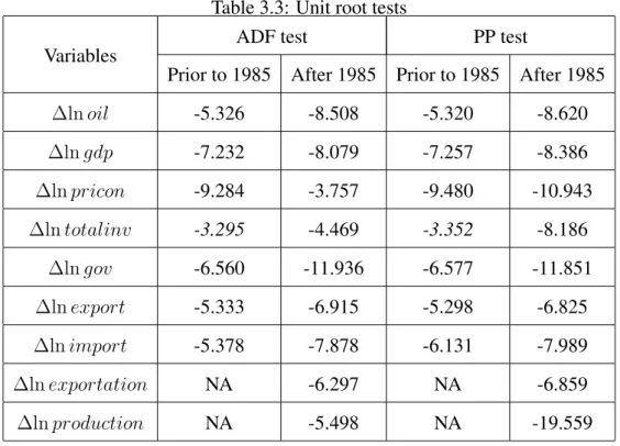
Prior to developing the structural VAR model, the unit root tests of these stochastic se-ries are first examined using two methods: Augmented Dickey-Fuller and Phillips-Perron methods. The null hypothesis is that the series has a unit root. If the null hypothesis is rejected, then this series will become stationary. The results of these unit root tests are listed in Table 3.3. The first-order differences of all logarithmic variables are stationary in our test results with these two methods for two sub-periods.
3.3.3
Structural Bivariate VAR Model
In empirical literature, the non-linear methods, DSGE and VAR models are used to study the effects of oil price shocks on macroeconomic aggregates. In the non-linear method, NOPIs are commonly used in research, such as in Hamilton (2009a, b). However, NOPIs only give the highest oil price level, and they cannot illustrate price fluctuations (e.g., cu-mulative change) in a given period. In reality, the effects of oil price shocks on economic activities do not only depend on the highest oil price level but also on the cumulative increase in oil prices over a given period (see Ferderer, 1996). In the DSGE model, the results of the simulation rely on the value of parameter. As we cannot cite the value of the parameter from other paper, writing a separate paper calibrating the parameter is required.
Table 3.3: Unit root tests Variables
ADF test PP test
Prior to 1985 After 1985 Prior to 1985 After 1985
∆ln oil -5.326 -8.508 -5.320 -8.620 ∆ln gdp -7.232 -8.079 -7.257 -8.386 ∆ln pricon -9.284 -3.757 -9.480 -10.943 ∆ln totalinv -3.295 -4.469 -3.352 -8.186 ∆ln gov -6.560 -11.936 -6.577 -11.851 ∆ln export -5.333 -6.915 -5.298 -6.825 ∆ln import -5.378 -7.878 -6.131 -7.989 ∆ln exportation NA -6.297 NA -6.859 ∆ln production NA -5.498 NA -19.559
Note: Italics are at 5% significant level, the others are at 1% significant level.
This paper adopts several bivariate VAR (i.e., oil price and one macroeconomic vari-able in the expenditure side of the national income) models. The theory support of adopt-ing this model to analyze this problem is that, for short sample periods and the small scale of oil price shocks, the effects of oil price shocks are linear, as demonstrated by Kilian and Vigfusson (2011). This model can fully describe the relationship between oil price shocks and the Japanese economy because the five variables in the expenditure side of the national income represent the economic structure of Japan. Note that, in Jimenez-Rodriguez and Sanchez (2005), their structural VAR model also includes long-term inter-est rate and short-term interinter-est rate. Our model only includes two variables. According to the results of Kilian (2009b), if oil price is ordered first in a bivariate model, that is, it is an exogenous variable, then the responses of macroeconomic aggregates to oil price shocks are assured asymptotically invariant to the inclusion of monetary policy ordered between oil price and macroeconomic aggregates. Moreover, if we adopt the Cholesky decom-position to simulate the structural VAR model, a variable of monetary policy should be placed after real GDP, as the government wants to smoothen the growth of the economy. Hence, the bivariate VAR model is useful and is the best methodology to be used.
The variables used in the model are ∆ln oil, ∆ln gdp, ∆ln pricon, ∆ln totalinv, ∆ln gov, ∆ln export, ∆ln import, and ∆ln exportation, ∆ln production. ∆ at the
be-ginning of all logarithmic variables is the first-order difference. The second half of each variable is the economic purport. Oil represents the real oil price of Japan’s case; gdp is Japan’s real GDP; pricon is private consumption; totalinv is the total investment; gov is the expenditure of government; export and import are the real mean in national income; exportation is the export of Japanese automobiles; and production is the production of Japanese automobiles.
Structural bivariate VAR models are used in the dynamic equation. The representative processes for the two sub-periods are as follows:
A0Yt = B0+ p X i=1 BiYt−i+ ut, (3.1) M0Yt = N0+ q X i=1 NiYt−i+ vt, (3.2)
where Yt = (y1, y2)0 is a (2×1) vector of ∆ln oil and one macroeconomic aggregate of
our interest; B0 and N0 are a (2×1) vector of intercept terms; A0 and M0, Bi and Ni
are (2×2) coefficient matrices; p and q are the optimal length of lags of each model; and ut and vt are white noise error vectors with zero mean and non-singular
variance-covariance matrix Σu and Σv, respectively. In Kilian (2008a) and Kilian (2009a), the
author selects 4 and 24 lags as the optimal length for his sample period, respectively. If we only observe the impulse response of one macroeconomic aggregate of our interest to oil price shocks, then high order lags can be tried in this model until we find higher order lags that contribute negligible amounts to the impulse response functions. The optimal length of each equation for our sample period is listed in Table 3.4.
In all structural VAR models, oil price is first considered as an exogenous variable to ensure that oil price shocks are not concurrently affected by changes of other macroeco-nomic aggregates. In fact, any VAR(p) model can be changed into a VAR(1) model, and the OLS method is used to estimate it. When calculating the impulse response functions of this model, we change the model into a vector moving average (∞) model.
Lee and Ni (2002) show that oil price shocks affect all economic sectors differently. Based on the variables in vector Yt, the effects of oil price shocks on the Japanese
econ-omy are analyzed in four steps. Step 1 analyzes the relationship between oil price shocks and real GDP. In Step 2, to explain the results in Step 1, five macroeconomic aggregates in the expenditure side of the national income (i.e., private consumption, total investment,
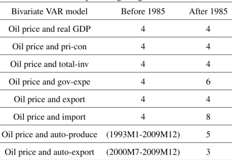
Table 3.4: The optimal lags length of each model
Bivariate VAR model Before 1985 After 1985
Oil price and real GDP 4 4
Oil price and pri-con 4 4
Oil price and total-inv 4 4
Oil price and gov-expe 4 6
Oil price and export 4 4
Oil price and import 4 8
Oil price and auto-produce (1993M1-2009M12) 5
Oil price and auto-export (2000M7-2009M12) 3
Table 3.5: The one standard deviation of oil price in each model
Bivariate VAR model Before 1985 After 1985
Oil price and real GDP 0.090331 0.146867
Oil price and pri-con 0.083325 0.149568
Oil price and total-inv 0.099061 0.149972
Oil price and gov-expe 0.098361 0.149010
Oil price and export 0.101207 0.150016
Oil price and import 0.093836 0.148995
Oil price and auto-produce (1993M1-2009M12) 0.083168 Oil price and auto-export (2000M7-2009M12) 0.089702
government expenditure, exports, and imports) must be enumerated first in detail. In Step 3, the different sectors and industries in the Japanese economy, which are affected by oil price shocks (e.g., automobile exports and production), are considered in more detail. Fi-nally, we explain the total responses of the Japanese economy using the weights of each term in the expenditure side of the national income (Step 4).
3.3.4
Empirical Results
Figures 3.3, 3.4, and 3.5 show the results of Steps 1, 2, and 3, respectively. The results show the estimated impulse response functions using one standard deviation of change in oil price. The magnitude of one standard deviation for each model is listed in Table 3.5. The dotted line in the following figures denotes the 95% confidence interval. The standard errors are calculated using the asymptotic method.
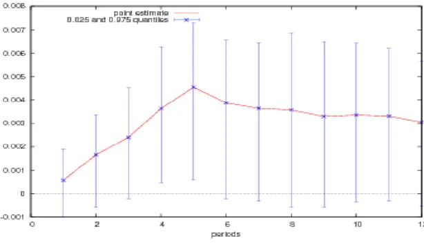
Figure 3.3: IRFs of Real GDP to oil price shocks
(The dotted line in the following figures is the 95% confidence interval)
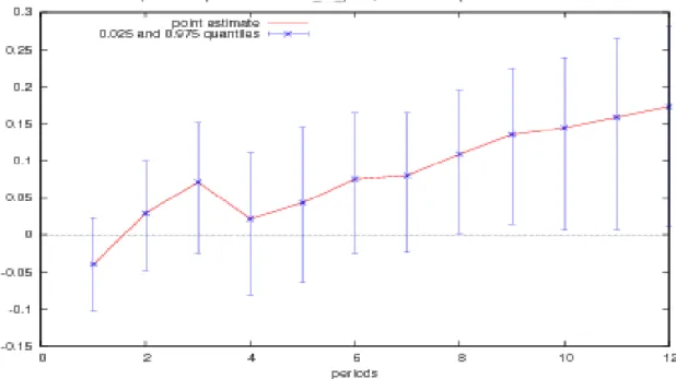
Figure 3.4: IRFs of expenditure side of national income to oil price shocks
Figure 3.5: IRFs of export and production of automobile to oil price shocks
(The dotted line in the following figures is the 95% confidence interval)
a aThe period of export is 2000M7-2009M12;
a aThe period of production is 1993M1-2009M12.
Step 1 shows two facts. First, consistent with typical reactions to oil price shocks, the Japan’s real GDP decreased before 1985 in Figure 3.3. The two oil price crises in the 1970s brought significant adverse effects to the Japanese economy. In contrast, Japan’s real GDP was almost unaffected over time after 1985. Second, similar to the results of Blanchard and Gali (2007), response scales in the Japanese economy became smaller after 1985.
The reason behind the insignificant change in Japan’s real GDP relative to oil price shocks is considered in Step 2. Henceforth, each term in the expenditure side of the national income is analyzed to explain the characteristics of the Japanese economy
Figure 3.4 shows the results on private consumption, total investment, government ex-penditure, and exports and imports in Step 2. Total investment includes private residential and non-residential investments, private and public inventories, and public investment in Japan’s case.
As seen in the first row on the left-hand side of Figure 3.4, prior to 1985, consumers simultaneously lowered their consumption levels because of anticipated decreases in fu-ture income. In the second row on the left-hand side of Figure 3.4, firm investments only show a small negative effect by oil price shocks. Government expenditure is not affected by oil price shocks in the first four quarters shown in the third row on the left-hand side of Figure 3.4. Consumer demand decreased and the Japanese yen depreciated during the period; hence, imports decreased accordingly, as evident in the fifth row on the left-hand side of Figure 3.4. These responses can be explained by empirical literature, such as Barsky and Kilian (2004) and Rotemberg and Woodford (1996).
The unique increase in Japan’s export sector relative to oil price shocks can be seen in the fourth row on the left-hand side of Figure 3.4. Since the 1970s, Japanese automo-biles have entered the international market and have become an important component of Japan’s export business. The series of energy and environmental laws passed in the US since 1980 has objectively promoted the importation of Japanese energy-efficient auto-mobiles in the country, as discussed in Hamilton (2009b).
However, our real interest is on why Japan’s real GDP was not affected after 1985. Private consumption of Japan was not significantly affected by the oil price shocks, as shown in the first row on the right-hand side of Figure 3.4, because there was no antic-ipated change in the future income. However, surprisingly, the total investment shows a
constant increase in the second row on the right-hand side of Figure 3.4. This characteris-tic of Japan’s economy is the most important after 1985. Government spending decreased to small levels, as shown in the third row on the right-hand side of Figure 3.4. Exports after 1985 particularly became larger than those were before 1985, as shown in the fourth row on the right-hand side of Figure 3.4. Recently, imports have experienced a slight increase, as shown in the fifth row on the right-hand side of Figure 3.4.
Why did firms choose to boost their investments during the oil price shocks after 1985? In the case of the US, the total investment increased, including the infrastructure and equipment investment of firms. This finding corresponds to the response of American firms, as the investment in the oil-mining sector also increased (Edelstein and Kilian, 2007). However, despite the fact that it has no oil-mining sector, why did Japans total investment also increase?
Figure 3.6: The growth rate of total investment and export before 1986
Note that Japanese exports increased in both sub-periods. Is there a correlation be-tween total investment and exports? Figures 3.6 and 3.7 plot the relationship of total investment and exports. Prior to 1986, an obvious relationship was not evident, as shown in Table 3.6, but after 1986, the Granger causality relationship already began, as shown in Table 3.7. When exports increase, firms will spend more money in investment. Corre-spondingly, when firm investments increase, Japanese export will also increase.
Table 3.6: Granger causality test total investment and exports from 1973 to 1985
Null Hypothesis F-statistic Prob
∆ln export dose not Granger cause ∆ln inv 0.85877 0.5183 ∆ln inv dose not Granger cause ∆ln export 1.27703 0.2958
Table 3.7: Granger causality test total investment and exports from 1986 to 2010
Null Hypothesis F-statistic Prob
∆ln export dose not Granger cause ∆ln inv 4.00254 0.0051 ∆ln inv dose not Granger cause ∆ln export 3.75796 0.0074
Next, we should determine which export sector increases during oil price shocks. Au-tomobile exports have the largest share in Japan’s total exports (18.4% in 1988 and 17.1% in 2007 based on trade statistics of Japan); hence, the automobile sector can be considered an important factor in Step 3. Figure 3.5 shows the trend of Japanese automobile exports and production for different periods, respectively, both of which exhibit an increase during oil price shocks. This result is in accordance with that of Hamilton (2009b).
Note that quarterly data are the shortest frequency data to describe macroeconomic aggregates in primary statistics. They are appropriate frequencies for portraying impulse-response functions in Figures 3.3 and 3.4. As regards the automobile sector of Japan, the Japan Automobile Manufacturers’ Association has counted automobile production since 1990s with monthly frequency. This sector is easily affected by market condition, such as price of gasoline, so monthly data are the best index to be used. Hamilton (2009b)
also uses monthly data to investigate this problem. The use of monthly frequency data to obtain the impulse-response functions is appropriate, as shown in Figure 3.5.
Table 3.8 shows the average weights of the expenditure side of the national income for the two periods in the Japanese economy. The weights of private consumption and total investment decreased, whereas the weights of expenditure of government, export, and import increased in the second sub-period. Moreover, the positive responses of total investment and export offset the negative response of government expenditure, which only created very minimal effects on Japan’s real GDP (Step 4).
Table 3.8: The each term weights in expenditure side of national income period Pri-consumption Total-inv Gov-expenditure Export Import
1973-1985 0.5968 0.2918 0.1031 0.0923 0.0830
1986-2010 0.5632 0.2591 0.1613 0.1041 0.0877
The reasons behind the weaker responses in Japan’s real GDP can be explained us-ing three factors, namely, the positive response of investment after 1985, the increase in Japanese (automobile) exports, and the low government expenditure in the expenditure side of the national income even if it has a negative response.
3.4
Two Frameworks of Economic Theory
An important finding of this study is the increase in total investment after 1986 in Japan’s case. Although the Granger causality between total investment and export in the Japanese economy exists, we are keen to know the transmission mechanisms of oil price shocks under this special phenomenon.
In the partial equilibrium analysis, Bernanke (1983) shows that the firm will imme-diately invest to avoid higher cost in the future if the increase in oil prices is permanent. Figure 3.8 shows the evolution of growth rate of oil price from 1960 to 2010. Before 1985, oil price trends were marked by sudden spikes, only showing a positive growth rate in a short time and then remaining at a constant level. After 1985, the change in oil prices became permanent.
Figure 3.8: The growth rate of oil price
Plante and Traum (2011) propose a general equilibrium analysis with a stochastic volatility of oil price to illustrate the theoretical relationship between real GDP, private consumption, investment, and oil price volatility. They find that total investment will increase because “the increase in oil price uncertainty has an impact on the uncertainty surrounding future income, and precautionary saving dominates as household investment in response to greater income uncertainty” if a country has no domestic oil-mining sector just like Japan.
3.5
Conclusions
This paper organizes the three types of oil prices and oil price shocks. Three kinds of structural bivariate VAR models are used, including oil price shocks and macroeconomic aggregates, to explain the effects of oil price shocks on Japan’s real GDP from 1973 to 2010.
In our four steps, we confirm the effects of oil price shocks on Japan’s real GDP and inspect the responses of each term in the expenditure side of the national income to the Japanese economy. If a positive movement in total investment is observed, the Granger causality between total investment and exports, as well as the frameworks of economic theory (i.e., partial and general equilibrium analysis) can explain this phenomenon. We also find that automobile export, which holds the largest share in the Japan’s export sector, increases as oil price increases. Lastly, we find that the government expenditure and imports have low shares in the expenditure side of the national income. We explain why
the effects of oil price shocks on Japan’s real GDP are not significant after 1985 through the responses of each term.
Japan, as a net oil-importing country, focuses on efficient energy use in its automobile industry. Once oil price shocks occur, export and production of automobiles increase. Moreover, Granger causality exists between the total investment and exports after 1985. These phenomena are unique features of the Japanese economy.
Data Sources
Items Sources
WTI EIA
World production of crude oil EIA
Japan’s automobile exports (2000M7-2009M12) JAMA
Japan’s automobile production (1993M1-2009M12) JAMA
Japan’s real national income Japan’s Cabinet Office
Exchange rate of Yen to US dollar International Monetary Fund
Japan’s CPI before 1980 International Monetary Fund
Japan’s CPI after 1980 STAT
Note: EIA is the Energy Information Administration. Japan’s real national income is season adjusted; JAMA is Japan Automobile Manufacturers Association. STAT is the website of Statistics Bureau, Director-General for Policy Planning (Statistical Standards) & Statistical Research and Training Institute, the address of this website is www.stat.go.jp.
Chapter 4
The Role of China’s Real Economic
Activity in Oil Price Changes
4.1
Introduction
Until now, we have known the effects of oil price shcoks on macroeconomic aggregates. In greater detail, oil price shocks can bring negative effects, such as inflation and reces-sion, on the majority oil importing countries. From now on, we study the causes of oil price changes.
A common viewpoint exists on the factors contributing to the increase in real oil price, that is, the supply shortage in the international market is attributable to the war or poltical strife in the Middle East before the 2000s. However, since 2002, no discernible reduction in crude oil production was observed. The only fact that stood out was the increase in real oil price. During the same period, a remarkable event in the international market in relation to crude oil is the rapid economic growth of Brazil, Russia, India and China (BRIC), all of which consumed large amounts of oil. As the largest economy among the BRIC countries, close attention is directed toward the role of China’s real economic activity on the increase in the real price of oil.
Hamilton (2009a, b), Frenkel and Rose (2010), and Kilian and Hicks (2011) argued that the strong demand for crude oil from high-growth industries in the Chinese economy is an important factor contributing to the increase of oil prices. By contrast, Du et al. (2010) suggested that the economic activity in China has no significant effect on the world oil price. This result was obtained using a Granger causality test. However, Du et al.
(2010) only used a reduced-form structural vector autoregression (VAR) model that has less stringent persuasion. In fact, Hamilton (2009a, b) and Kilian and Hicks (2011) have not directly tested and verified the effects of China’s economic activity as a single variable on oil price variability. For instance, Hamilton (2009a, b) only provided the absolute quantity and growth rate of oil consumption in China, but did not calculate its effects on the real price of oil. On the other hand, Kilian and Hicks (2011) focused only on two countries (China and India) as one unit in analysing this problem.
The current study is motivated by the need to confirm whether the Chinese economy has affected the real price of oil in recent decades. In determining this effect, the present work used a structural VAR model and found that shocks in the oil market-specific and Organisation for Economic Cooperation and Development (OECD) demands imposed considerable effects on the real price of crude oil from 1994 to 2010. In addition, prior to 2002, China’s real economic activity had no power to affect the real price of oil. From 2002, however, the demand shocks resulting from China’s economic activity positively af-fected world oil price, but this effect remains temporary and minimal. Until 2010, China’s oil consumption accounted for a very small proportion of the world’s total consumption, suggesting the reasons for the minimal effect of the Chinese economy on the real price of oil. The effect of China’s real economic activity on the real price of oil may be important in the future, but not at the present time. To obtain accurate results, a different software program was used in the present work for the simulation of this process.
The remainder of the current chapter is organised as follows: Subsection 4.2 sum-marises prior research on oil price shocks and economic activity. Subsection 4.3 clarifies a number of basic problems before discussing the structure of the proposed model. Sub-section 4.4 presents the econometric model and its identifying restrictions. SubSub-section 4.5 provides the analysis of the empirical results and emphasises the role of four types of shock (one supply and three demand shocks) on the three applications of the structural VAR model. Subsection 4.6 then concludes.
4.2
Literature Review
Between 2003 and middle of 2008, crude oil prices surged in the international market, an event that concerned economists and prompted them to revisit the fundamental issues