under a monotone incomplete sample

1 Introduction

There are situations where some variates are missing in multivariate statistical analysis, for example, some of the variables to be measured are too expensive. The problem of missing data is an important applied problem. For analyzing these data, various statistical methods have been developed by Anderson [1], Anderson and Olkin [2], Dempster, Laird and Rubin [5], Srivastava [13] and Little and Rubin [9].

In this paper, we consider ak-step monotone incomplete sample. Let x be distributed as Np(ñ;Ü), andx⁽ⁱ⁾ the vector of the årstqielements ofx, wherep=q1 > q2 >ÅÅÅ> qk>0.

We partitionxas

x= (x⁰₁; : : : ;x⁰_k)⁰; xi:piÇ1;

andp1+ÅÅÅ+pi=q_kÄi+1fori= 1; : : : ; k. Then

x⁽¹⁾= (x⁰₁; : : : ;x⁰_k)⁰;x⁽²⁾= (x⁰₁; : : : ;x⁰_kÄ1)⁰; : : : ;x^(k)=x1:

Suppose that we haveN1observations on x⁽¹⁾,N2 observations onx⁽²⁾, and so on. Letx⁽ⁱ⁾_j be the j-th observation onx⁽ⁱ⁾. Here it is assumed that the marginal density function of the observed data setfx⁽¹⁾₁ ; : : : ;x⁽¹⁾_N1; : : : ;x^(k)₁ ; : : : ;x^(k)_Nk;gis

Yk i=1

Ni

Y

j=1

f(x⁽ⁱ⁾_j jñ_[i];Ü(1;:::;i)(1;:::;i)); (1)

wheref(x⁽ⁱ⁾_j jñ_[i];Ü(1;:::;i)(1;:::;i)) is the density function ofNqkÄi+1

êñ_[i];Ü(1;:::;i)(1;:::;i)

ë and

ñ_[i]= 0 BB BB

@ ñ₁ ñ₂ ... ñ

1 CC CC

A; Ü(1;:::;i)(1;:::;i)= 0 BB BB

@

Ü₁₁ Ü₁₂ ÅÅÅ Ü_1i Ü21 Ü22 ÅÅÅ Ü2i

... ... . .. ...

Ü Ü ÅÅÅ Ü

1 CC CC A; Abstract

In this article, we consider an inference for a covariance matrix under monotone incom- plete sample. The maximum likelihood estimator for a mean vector is unbiased but that of the covariance matrix is not unbiased. We derive an unbiased estimator for the covari- ance matrix using some fundamental properties of Wishart matrix. The accuracy of the estimators is investigated by numerical simulation.

1

TSUKADA Shin-ichi

Unbiased estimators for the covariance matrix

under a monotone incomplete sample

whereñ_j is apj-dimensional vector and Üjlis a (pj; pl) matrix.

Anderson and Olkin [2] consider the 2-step monotone sample and derive the maximum like- lihood estimator(MLE) ^ñand ^Ü for the mean vectorñand the covariance matrix Ü based on the density function (1). Fujisawa [6] has obtained the estimators by the conditional approach.

Kanda and Fujikoshi [8] investigate some fundamental properties of the MLE, and indicate that the MLE ^ñfor the mean vector is unbiased but the MLE ^Ü for the covariance matrix is not unbiased. In general, it becomes diécult to derive the exact properties of these estimators ex- cept for some special cases. They study the asymptotic properties. Chang and Richards [3], [4]

derive a stochastic representation for the exact distribution of the MLE ^ñand ^Ü under the 2-step monotone sample. They obtain ellipsoidal conådence region forñand deal with the hypothesis testing for the covariance matrix. Provost [11] considers the mutual independence of covariance matrix under the 2-step monotone incomplete sample and derives the likelihood ratio criterion.

Hao and Krishnamoorthy [7] deal with the hypothesis testing that the covariance matrix is equal to a speciåed matrix and that the mean vector and the covariance matrix equal to a given vec- tor and matrix under thek-step monotone incomplete sample. They derive the likelihood ratio criteria and asymptotic null distribution.

Fork = 2 or k= 3, we derive an unbiased estimator for the covariance matrix using some fundamental properties by Kanda and Fujikoshi [8]. We deal with the 2-step and the 3-step monotone incomplete sample in Section 2 and 3, respectively. In Section 4, the accuracy of the unbiased estimators is investigated by numerical simulation.

2 2-step monotone incomplete data

Let thep-dimensional variate xbe decomposed as (x⁰₁;x⁰₂), wherex1 andx2 arep1 andp2- dimensional vectors, respectively. Suppose that we haveN1 observations on the full set of vari- ables, i.e.,x, andN2observations onx1, and these observations are independently distributed.

That is, we have the following observations:

† x11

x21

!

;

† x12

x22

!

;ÅÅÅ

† x1N1

x2N1

!

;

† x1N1+1

É

!

;ÅÅÅ

† x1N1+N2

É

! :

Let ñx⁽¹⁾denote the sample mean ofxbased on theN1observations, and ñx⁽¹⁾= (ñx⁽¹⁾₁ ⁰;xñ⁽¹⁾₂ ⁰)⁰, ñ

x⁽¹⁾_i : piÇ1. Let ñx⁽²⁾ denote the sample mean of thep1-dimensional elements ofx1 based on the N2 observations. Throughout this article, we use the letter ãonly as running suéx for sample observations. Then the sample covariance matrix based on theN1andN2observations are expressed as

S⁽¹⁾= 1 n1

N1

X

ã=1

(x⁽¹⁾_ã Äxñ⁽¹⁾)(x⁽¹⁾_ã Äxñ⁽¹⁾)⁰; S⁽²⁾= 1 n2

N2

X

ã=1

(x⁽²⁾_ã Äxñ⁽²⁾)(x⁽²⁾_ã Äxñ⁽²⁾)⁰;

respectively, whereni=NiÄ1,i= 1;2. Let the partitions ofñ, Ü andS⁽¹⁾ corresponding to the ones ofxbe

ñ=

† ñ₁ ñ₂

!

; Ü =

† Ü11 Ü12

Ü21 Ü22

!

; S⁽¹⁾=

† S₁₁⁽¹⁾ S₁₂⁽¹⁾ S₂₁⁽¹⁾ S₂₂⁽¹⁾

! :

2.1 Maximum likelihood estimator

Let the maximum likelihood estimator ofñand Ü denote by ^ñand ^Ü, respectively, which are partitioned in the same way asñand Ü. We can represent ^ñand ^Ü as follows:

^ ñ₁= 1

N

êN1xñ⁽¹⁾₁ +N2xñ⁽²⁾ë

; ñ^₂= ñx⁽¹⁾₂ ÄÜ^21Ü^^Ä1₁₁ ê ñ x⁽¹⁾₁ Äñ^₁ë

; Ü^11= 1

N

êW₁₁⁽¹⁾+W⁽²⁾ë

; Ü^12= ^Ü11

êW₁₁⁽¹⁾ëÄ1

W₁₂⁽¹⁾; Ü^22= 1

N1W_22Å⁽¹⁾₁+ ^Ü21Ü^^Ä₁₁¹Ü^12; (2) whereN=N1+N2,

W⁽¹⁾=n1S⁽¹⁾; W⁽²⁾=n2S⁽²⁾+N1N2

N

êxñ⁽¹⁾₁ Äxñ⁽²⁾ë ê ñ

x⁽¹⁾₁ Äxñ⁽²⁾ë0

; W⁽¹⁾=

† W₁₁⁽¹⁾ W₁₂⁽¹⁾ W₂₁⁽¹⁾ W₂₂⁽¹⁾

!

; W_22Å⁽¹⁾₁=W₂₂⁽¹⁾ÄW₂₁⁽¹⁾ê

W₁₁⁽¹⁾ëÄ1

W₁₂⁽¹⁾:

Kanda and Fujikoshi [8] prove the following lemma which is useful in deriving the expectation and variance of ^ñand ^Ü.

Lemma 2.1. Suppose thatAis distributed as a Wishart distributionWp(Ü; n)andnïp, where Ais partitioned as in the partition ofÜ, and letA_22Å1=A22ÄA21A^Ä1₁₁A12. Then we have

(i) A_22Å1òWp2(Ü_22Å1; nÄp1), andA_22Å1is independent ofA11andA12,

(ii) The conditional distribution of vec(A12) given A11 is distributed as normal distribution with the mean vectorvec(A11Ü^Ä1₁₁Ü12)and the covariance matrixÜ_22Å1äA11. In particular E[A^Ä1₁₁A12] = Ü^Ä1₁₁Ü12, where vec(C) denotes the column vector formed by stacking the columns of C under each other,

(iii) A11òWp1(Ü11; n),

(iv) ifnÄpÄ1>0, thenE[A^Ä1] = 1 nÄpÄ1Ü^Ä1

(v) ifnÄpÄ1>0, thenE[A21A^Ä1₁₁CA^Ä₁₁¹A12] =E[trA^Ä1₁₁C]Ü_22Å1+ Ü21Ü^Ä1₁₁E[C]Ü^Ä1₁₁Ü12; whereC is a random matrix depending onA11.

Proof. The results from (i) to (iv) are well known. For a proof, see Muirhead[10] and Siotani, Hayakawa and Fujikoshi[12]. The result (v) follows from (ii) and (iv).

Using the above lemma, the expectation and variance of ^ñ and the expectation of ^Ü are obtained as follows:

Theorem 2.1(Kanda and Fujikoshi [8]). Suppose thatN1> p. Then the mean and the covari- ance matrix ofñ^ and the mean ofÜ^ are given by

(i) E[^ñ] =ñ, (ii) Var[^ñ] = 1

N

† Ü11 Ü12

Ü₂₁ NVar[^ñ₂]

!

; (N1> p1+ 2), where

Var[^ñ₂] = 1 N1

í

Ü22ÄN2

NÜ21Ü^Ä₁₁¹Ü12

ì

+ N2p1

N N1(N1Äp1Ä2)Ü_22Å1;

(iii) E[ ^Ü] =NÄ1 N Ü + 1

N

† O O

O b0Ü_22Å1

!

;

where

b0=ÄN2fN1Ä(p1+ 1)(p1+ 2)g N1(N1Äp1Ä2) :

Proof. The results for the mean vector are derived by using ñx⁽¹⁾ ò N(ñ; N₁^Ä1Ü), ñx⁽²⁾ ò N(ñ₁; N₂^Ä1Ü11) and Lemma 2.1. The result for the covariance matrix is derived by using W⁽¹⁾ ò W_p(Ü; N₁Ä1), W⁽²⁾ ò W_p1(Ü₁₁; N₂), and Lemma 2.1 and thatW⁽¹⁾ and W⁽²⁾ are independently distributed.

We may see that ^ñis unbiased and ^Ü is biased. Kanda and Fujikoshi [8] recommend a usual correction

Ü =~ N

NÄ1Ü^ (3)

for an estimator of Ü. In the next subsection, we will obtain the unbiased estimator of Ü.

2.2 Unbiased estimator of covariance matrix

From Theorem 2.1, the MLE ^Ü of the covariance matrix is biased. In this section, we obtain the unbiased estimator for Ü as follows.

Theorem 2.2. Let

~~Ü =

† Ü~11 Ü~12

Ü~21 ~~Ü22

!

; (4)

where

~~Ü22= ~Ü22Äc0Ü^_22Å1; c0= N2(p1+ 1)(p1+ 2)ÄN1N2

(NÄ1)(N1Äp1Ä2)(N1Äp1Ä1): Suppose thatN1>max(p; p1+ 2). Then we have

Eh

~~Üi

= Ü:

Proof. Since it is trivial thatEh Ü~11

i= Ü11,Eh Ü~12

i= Ü12 andEh Ü~21

i= Ü21, we prove that

Eh

~~Ü₂₂i

= Ü22. It follows from Theorem2.1 (iii) that

Eh Ü~22

i = í

1 + b0

NÄ1 ì

Ü22Ä b0

NÄ1Ü21Ü^Ä1₁₁Ü12: (5) Using the equation (2), the estimator ^Ü21Ü^^Ä₁₁¹Ü^12is written as follows:

Ü^21Ü^^Ä1₁₁Ü^12 = 1 NW₂₁⁽¹⁾ê

W₁₁⁽¹⁾ëÄ1

W₁₂⁽¹⁾+ 1 NW₂₁⁽¹⁾ê

W₁₁⁽¹⁾ëÄ1

W⁽²⁾ê W₁₁⁽¹⁾ëÄ1

W₁₂⁽¹⁾: Since

E î

W₂₁⁽¹⁾ê W₁₁⁽¹⁾ëÄ1

W₁₂⁽¹⁾ ï

=p1Ü22+ (N1Äp1Ä1)Ü21Ü^Ä1₁₁Ü12;

E î

W₂₁⁽¹⁾ê W₁₁⁽¹⁾ë_Ä1

W⁽²⁾ê W₁₁⁽¹⁾ë_Ä1

W₁₂⁽¹⁾ ï

= N₂p₁

N₁Äp₁Ä2Ü22+N₂(N₁Ä2p₁Ä2)

N₁Äp₁Ä2 Ü21Ü^Ä1₁₁Ü12

from Lemma2.1, one sees that Eh

Ü^21Ü^^Ä₁₁¹Ü^12

i = p1

N

NÄp1Ä2

N1Äp1Ä2Ü22+ B0

N(N1Äp1Ä2)Ü21Ü^Ä1₁₁Ü12; (6) where

B0=N₁²+N1(N2Ä2p1Ä3)Ä(p1+ 1)(2N2Äp1Ä2):

From Theorem2.1 (iii), (5) and (6), we obtain that Eh

~~Ü22

i=Eh Ü~22

iÄc0Eh Ü^22

i+c0Eh

Ü^21Ü^^Ä1₁₁Ü^12

i= Ü22:

The eãect of the unbiasedness is investigated by the numerical simulation in Section 4.

3 3-step monotone incomplete data

As in Section 2, we consider the case of the 3-step monotone incomplete sample. Let the p-dimensional variatexbe decomposed as (x⁰₁;x⁰₂;x⁰₃), wherex1,x2andx3arep1,p2andp3- dimensional vectors, respectively. Suppose that we haveN1observations onx,N2observations on (x⁰₁;x⁰₂)⁰, andN₃observations onx₁, and that these observations are independently distributed.

That is, we have the following observations:

0 B@

x11

x21

x₃₁ 1 CA;ÅÅÅ;

0 B@

x1N1

x2N1

x_3N1 1 CA;

0 B@

x1N1+1

x2N1+1

É 1 CA;ÅÅÅ;

0 B@

x1N1+N2

x2N1+N2

É 1 CA;

0 B@

x1N1+N2+1

É É

1 CA;ÅÅÅ;

0 B@

x1N1+N2+N3

É É

1 CA:

Let ñx⁽¹⁾= (ñx⁽¹⁾₁ ⁰;xñ⁽¹⁾₂ ⁰;xñ⁽¹⁾₃ ⁰)⁰denote the sample mean ofxbased on theN1observations, and ñ

x⁽²⁾ = (ñx⁽²⁾₁ ⁰;xñ⁽²⁾₂ ⁰)⁰ denote the sample mean for the årst (p1+p2)-dimensional elements ofx based on theN2observations, respectively, and ñx⁽³⁾denote the sample mean forp1-dimensional elements ofx1based on theN3observations. The corresponding sample covariance matrices are denoted byS⁽ⁱ⁾(i= 1;2;3) as follows:

S⁽¹⁾ = 1 n1

N1

X

ã=1

(x⁽¹⁾_ã Äxñ⁽¹⁾)(x⁽¹⁾_ã Äxñ⁽¹⁾)⁰;

S⁽²⁾ = 1 n2

N2

X

ã=1

† x⁽²⁾_1ãÄxñ⁽²⁾₁ x⁽²⁾_2ãÄxñ⁽²⁾₂

! † x⁽²⁾_1ãÄxñ⁽²⁾₁ x⁽²⁾_2ãÄxñ⁽²⁾₂

!0

; S⁽³⁾ = 1

n3 N3

X

ã=1

(x⁽³⁾_ã Äxñ⁽³⁾)(x⁽³⁾_ã Äxñ⁽³⁾)⁰; whereni=NiÄ1; (i= 1;2;3) andN=N1+N2+N3.

Let the partitions ofñand Ü corresponding to the ones ofxbe

ñ= 0 B@

ñ₁ ñ₂ ñ₃

1 CA; Ü =

0 B@

Ü11 Ü12 Ü13

Ü21 Ü22 Ü23

Ü31 Ü32 Ü33

1 CA=

† Ü(12)(12) Ü(12)3

Ü3(12) Ü33

! :

Similar partitions and notations are used forS⁽ⁱ⁾and for other matrices.

3.1 Maximum likelihood estimator

We can represent ^ñand ^Ü as follows:

ñ^₁ = 1 N

êN1xñ⁽¹⁾₁ +N2xñ⁽²⁾₁ +N3xñ⁽³⁾ë

;

^

ñ₂ = 1 N1+N2

êN1xñ⁽¹⁾₂ +N2xñ⁽²⁾₂ ë ÄF⁰

†N1xñ⁽¹⁾₁ +N2xñ⁽²⁾₁ N1+N2 Äñ^₁

!

;

ñ^₃ = xñ⁽¹⁾₃ ÄG⁰

† xñ⁽¹⁾₁ Äñ^₁ ñ x⁽¹⁾₂ Äñ^₂

!

; Ü^11 = 1

N

êW₁₁⁽¹⁾+W₁₁⁽²⁾+W⁽³⁾ë

; Ü^12= ^Ü11F;

Ü^22 = 1 N1+N2

êW_(12)(12)⁽¹⁾ +W⁽²⁾ë

22Å1+F⁰Ü^11F;

Ü^(12)3 = Ü^(12)(12)G; Ü^33= 1

N1W_33Å⁽¹⁾₁₂+G⁰Ü^(12)(12)G;

where

F = ê

W₁₁⁽¹⁾+W₁₁⁽²⁾ë_Ä1ê

W₁₂⁽¹⁾+W₁₂⁽²⁾ë

; G=ê

W_(12)(12)⁽¹⁾ ë_Ä1 W₍₁₂₎₃⁽¹⁾ ; W⁽¹⁾ = n₁S⁽¹⁾;

W⁽²⁾ = n2S⁽²⁾+ N1N2

N1+N2

† xñ⁽¹⁾₁ Äxñ⁽²⁾₁ ñ x⁽¹⁾₂ Äxñ⁽²⁾₂

! † xñ⁽¹⁾₁ Äxñ⁽²⁾₁ ñ x⁽¹⁾₂ Äxñ⁽²⁾₂

!₀

;

W⁽³⁾ = n3S⁽³⁾+(N1+N2)N3

N ö

ñ

x⁽³⁾Ä 1 N1+N2

êN1xñ⁽¹⁾₁ +N2xñ⁽²⁾₁ ëõ

Ç ö

xñ⁽³⁾Ä 1 N1+N2

êN1xñ⁽¹⁾₁ +N2xñ⁽²⁾₁ ëõ⁰ : The natural parameters in the conditional approach are deåned by

ë= 0 B@

ë₁ ë₂ ë₃

1 CA; Å =

0 B@

Å11 Å12 Å13

Å21 Å22 Å23

Å31 Å32 Å33

1 CA;

which are one to one correspondence to (ñ;Ü), where

Å11= Ü11; Å12= Å⁰₂₁= Ü^Ä1₁₁Ü12; Å22= Ü_22Å1= Ü22ÄÜ21Ü^Ä1₁₁Ü12; Å₍₁₂₎₃= Å⁰₃₍₁₂₎= Ü^Ä1_(12)(12)Ü₍₁₂₎₃;

Å33= Ü_33Å12= Ü33ÄÜ₃₍₁₂₎Ü^Ä1_(12)(12)Ü₍₁₂₎₃: The MLE (^ë;Å) of (ë;^ Å) are expressed as follows:

^

ë₁= ^ñ₁; ë^₂= ñx⁽¹⁾₂ ÄÅ^21xñ⁽¹⁾₁ ; ë^₃= ñx⁽¹⁾₃ ÄÅ^₃₍₁₂₎

† xñ⁽¹⁾₁ xñ⁽¹⁾₂

!

; Å^11= ^Ü11; Å^12= ^Å⁰₂₁=ê

W₁₁⁽¹⁾+W₁₁⁽²⁾ë_Ä1ê

W₁₂⁽¹⁾+W₁₂⁽²⁾ë

; Å^22= 1

N1+N2

êW_(12)(12)⁽¹⁾ +W⁽²⁾ë

22Å1; Å^₍₁₂₎₃=ê

W_(12)(12)⁽¹⁾ ëÄ1

W₍₁₂₎₃⁽¹⁾ ; Å^33= 1 N1W_33Å⁽¹⁾₁₂:

The following lemma is published in Kanda and Fujikoshi [8] to calculate the expectation and variance of ^ñand ^Ü.

Lemma 3.1. Suppose thatA, B andC is independently distributed as a Wishart distribution Wp(Ü; n1),Wp(Ü; n2)andWp(Ü; n3), respectively. Letn=n1+n2+n3 and letA,B,C andÜ be partitioned as in Lemma 2.1. Further, letL= (A11+B11)^Ä1(A12+B12), and let

D=

† D11 D12

D21 D22

!

;

whereD11=A11+B11+C11,D12=D⁰₂₁=D11L,D22=çA_22Å1+L⁰D11Landçis a constant.

Then we have (i) E[D11] =nÜ11, (ii) E[D₁₂] =nÜ₁₂,

(iii) ifn1+n2Äp1Ä1>0, then

E[D22] =ç(nÄp1)Ü_22Å1+nÜ21Ü^Ä1₁₁Ü12+p1

ö

1 + n₃

n1+n2Äp1Ä1 õ

Ü_22Å1, (iv) ifn₁ÄpÄ1>0, then

E[trA^Ä1D] =p1+çp2+(n2+n3)p1

n1Äp1Ä1+ p1p2

n1Äp1Ä1

í n2+n3

n1Äp1Ä1Ä n3

n1+n2Äp1Ä1 ì

(v) ifn1ÄpÄ1>0, then

E

"

trA^Ä1

† Ip1

L⁰

!

Ü₁₁(I_p1 L⁰)

#

= p1

n₁Äp₁Ä1 + p1p2

n1ÄpÄ1

í 1

n1Äp1Ä1Ä 1 n1+n2Äp1Ä1

ì : Proof. The results (i), (ii) and (iii) are easily obtained from Lemma 2.1. For (iv) and (v), we evaluate the expectation by three steps; (1) A_22Å1, (2) A12, B12, (3) A11,B11, C11 using the inverse matrix of the partition matrix. See Kanda and Fujikoshi [8] for details.

The expectation of ^Ü is obtained as follows:

Theorem 3.1(Kanda and Fujikoshi [8]). Suppose thatN₁> pandN₁> p₁+p₂+ 2. Then

Eh Ü^i

= NÄ1 N Ü + 1

N 0 B@

O O O

O B22 B23

O B32 B33

1

CA; (7)

whereB22=b1Ü_22Å1,B23=B₃₂⁰ =b1Ü_22Å1Å23,B33=b1Å32Ü_22Å1Å23+b2Ü_33Å12; b1 = ÄN3fN1+N2Ä(p1+ 1)(p2+ 2)g

N(N1+N2)(N1+N2Äp1Ä2); b₂ = Ä1

N

î(N2+N3)fN1Ä(p1+ 1)(p1+p2+ 2)g

N₁(N₁Äp₁Äp₂Ä2) + p2N N2

N₁(N₁+N₂)

+ p1p2N3

(N1Äp1Äp2Ä2)(N1+N2Äp1Ä2) ï

:

Proof. To proof this theorem, it is used thatW⁽¹⁾,W⁽²⁾andW⁽³⁾are independently distributed asWp(Ü; N1Ä1),Wp1+p2(Ü(12)(12); N2) andWp1(Ü11; N3), respectively. Lemma 2.1 and Lemma 3.1 are applied to evaluate the expectation. See Kanda and Fujikoshi [8] for details.

3.2 Unbiased estimator of covariance matrix

From Theorem 3.1, the MLE ^Ü of the covariance matrix is biased as well as the 2-step monotone incomplete sample. In this section, we obtain the unbiased estimator for Ü in the 3-step monotone incomplete sample.

Theorem 3.2. Let

~~Ü₂₂ = Ü~22Äc0Ü^_22Å1; ~~Ü_(12)(12)=

† Ü~11 Ü~12

Ü~21 ~~Ü₂₂

!

;

~~Ü₍₁₂₎₃ = ~~Ü_(12)(12)ê

W_(12)(12)⁽¹⁾ ëÄ1

W₍₁₂₎₃⁽¹⁾ ; ~~Ü₃₃=c1Ü^33+c2Å^32Ü^_22Å1Å^23+c3Ü^_33Å12; where

c0 = N b1

(NÄ1)(b1+d0); c1 = N

NÄ1Ä N²d1(N1Ä2)

(NÄ1)(d2Äd2NÄ2d1N+d1N N1); c2 = Ä b1(d1+d2)(N1+N2)

(N1+N2Äp1Ä1)fd2(NÄ1)ÄN d1(N1Ä2)g;

c3 = d1N

d2Äd2NÄ2d1N+d1N N1;

d0 = (N1+N2Ä1Äp1) +N3N1+N2Ä2p1Ä2p2Ä2 N1+N2Äp1Äp2Ä2 ; d₁ = b2(N1+N2Äp1Ä1)

N(N₁+N₂) Ä b1p2(N1+N2Äp1Äp2Ä2) N(N₁+N₂)(N₁Äp₁Äp₂Ä2); d2 = b1p2(N1+N2Äp1Äp2Ä2)

N(N1+N2)(N1Äp1Äp2Ä2):

Suppose thatN1> p,N2+ 1> p1+p2,N3+ 1> p3 andN1Äp1Äp2Ä2>0. Then we have E

"†

~~Ü_(12)(12) ~~Ü₍₁₂₎₃

~~Ü₃₍₁₂₎ ~~Ü33

!#

= Ü:

Proof. Here, some typical expectations needed to evaluate the expectation of unbiased estimator are shown, and details are omitted. Applying Lemma 2.1, we get

Eh

Ü^21Ü^^Ä1₁₁Ü^12

i= îNÄ1

N Ä 1 N

ö

(N1+N2Ä1Äp1) +N3N1+N2Ä2p1Ä2p2Ä2 N1+N2Äp1Äp2Ä2

õ ï Ü22

+1 N

ö

(N₁+N₂Ä1Äp₁) +N₃N1+N2Ä2p1Ä2p2Ä2 N₁+N₂Äp₁Äp₂Ä2

õ

Ü₂₁Ü^Ä1₁₁Ü₁₂:

We can evaluate the expectation of ~~Ü₂₂ using the above equation and Theorem 3.1.

The expectation of ~~Ü22 could be proved by a similar calculation for ^Ü₍₁₂₎₃in Theorem 3.1.

Eh

~~Ü₍₁₂₎₃i

= E

î~~Ü_(12)(12)ê

W_(12)(12)⁽¹⁾ ë_Ä1

W₍₁₂₎₃⁽¹⁾ ï

= Eh

~~Ü_(12)(12)i

Ü^Ä1_(12)(12)Ü₍₁₂₎₃

= Ü(12)(12)Ü^Ä1_(12)(12)Ü(12)3= Ü(12)3: Using Lemma 2.1 and Lemma 3.1, we get

Eh Ü^_33Å12

i = (N1Ä2)Ü33Äb1

NÅ32Ü_22Å1Å23

+ ö 1

N1(N1Äp1Äp2Ä1)Ä(N1Ä2) õ

Ü_33Å12;

Eh

Å^₃₂Ü^_22Å1Å^₂₃i

= (N1+N2Äp1Äp2Ä2)p2

(N1+N2)(N1Äp1Äp2Ä2)Ü_33Å12+N1+N2Ä1Äp1

N1+N2

Å₃₂Ü_22Å1Å₂₃:

The expectation of ~~Ü33 can be evaluated by the expectation of ^Ü33 in Theorem 3.1 and the above equations.

We see that the estimator

~~Ü =

† ~~Ü_(12)(12) ~~Ü₍₁₂₎₃

~~Ü₃₍₁₂₎ ~~Ü33

!

is unbiased. As well as the 2-step incomplete sample, the eãect of the unbiasedness is investigated by the numerical simulation in Section 4.

4 Numerical simulation

In this section, we evaluate the expectation of estimators by numerical simulation. LetT = (tij) be the estimator of covariance matrix, i.e., ^Ü, ~Ü and ~~Ü. The expectation of the estimator T is evaluated by

Tñ= (ñtij) = 1 ns

ns

X

i=1

Ti;

wherensis a number of simulation andTiis the estimator in each simulation. We adopt

E= Xp

i;j=1 iîj

(ñtijÄõij)²

as the diãerence between ñTand Ü = (õij). The number of simulation is a hundred thousand.

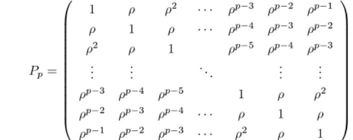
Let

Pp= 0 BB BB BB BB BB BB

@

1 ö ö² ÅÅÅ ö^pÄ3 ö^pÄ2 ö^pÄ1 ö 1 ö ÅÅÅ ö^pÄ4 ö^pÄ3 ö^pÄ2 ö² ö 1 ö^pÄ5 ö^pÄ4 ö^pÄ3

... ... . .. ... ...

ö^pÄ3 ö^pÄ4 ö^pÄ5 1 ö ö² ö^pÄ2 ö^pÄ3 ö^pÄ4 ÅÅÅ ö 1 ö ö^pÄ1 ö^pÄ2 ö^pÄ3 ÅÅÅ ö² ö 1

1 CC CC CC CC CC CC A :

As the population covariance matrix, we adopt the following matrices Ü1 = É1pPpÉ1p; (Case 1) Ü2 = É2pPpÉ2p; (Case 2)

where É1p= diag(õ^pÄ1; õ^pÄ2; : : : ; õ²; õ;1) and É2p=õIp, and assume that the population mean vector is0.

4.1 2-step monotone incomplete sample

We assume that the population distribution is the 7-variate normal distribution. Letp1 = 4 andp2 = 3. We setö= 0:15 and õ=p

2 in Case 1,ö= 0:5 andõ= 2 in Case 2. The total sample size are 50, 100, 200, 500 and 1000. The missing rateú(=N2=N) are 0.2, 0.4, 0.6, 0.8.

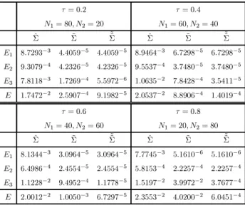
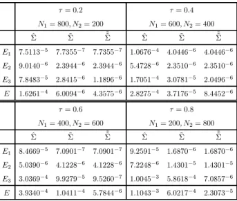
Table 1 represents the coeécientc0of the unbiased estimator. Table 2 - Table 6 represent the results in Case 1, and the results in Case 2 are represented in Table 7 - Table 11. In Table,E1, E2andE3 denote a partial error as follows:

E =

p1

X

i;j=1 iîj

(ñtijÄõij)²+

p1

X

i=1

Xp j=p1

(ñtijÄõij)²+ Xp i;j=p1+1

iîj

(ñtijÄõij)²ëE1+E2+E3;

which are the error for Ü11, Ü12 and Ü22, respectively, and the notationx^y denotes the value xÇ10^y.

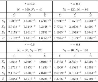
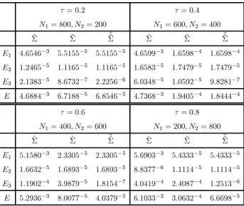
As a matter of course, errors are small when the total sample sizeN is large. The error of ~Ü and the unbiased estimator is smaller than that of the maximum likelihood estimator as a whole.

The error of ~Ü is close to that of the unbiased estimator in the case ofú= 0:2, but the error of the unbiased estimator is smaller than that of ~Ü inú= 0:8. There is a similar tendency in each Table, and the diãerence of errors is about one digit whenN= 1000.

From these results, it is obvious that the unbiased estimator is more accurate. We recommend this estimator under the 2-step incomplete sample.

4.2 3-step monotone incomplete sample

We set the parameters of the population distribution as well as under the 2-step monotone incomplete sample. It assumes that the population distribution is the 9-variate normal distribu- tion andp1=p2=p3= 3. We setö= 0:15 andõ=p

2 in Case 1,ö= 0:5 andõ= 2 in Case 2 as the 2-step monotone incomplete sample.

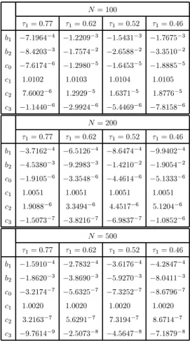
The missing rates (ú1; ú2; ú3) are (0.77, 0.15, 0.08), (0.62, 0.25, 0.13), (0.52, 0.32, 0.16) and (0.46, 0.36, 0.18). The coeécients concerning the unbiased estimator is represented in Table 12.

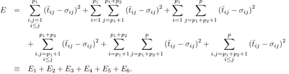
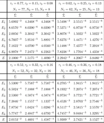
Table 13 - Table 15 represent the result in Case 1, and the results in Case 2 are represented in Table 16 - Table 18. In Table, fromE₁ toE₆denote a partial error as follows:

E =

p1

X

i;j=1 iîj

(ñtijÄõij)²+

p1

X

i=1 p1X+p2

j=p1+1

(ñtijÄõij)²+

p1

X

i=1

Xp j=p1+p2+1

(ñtijÄõij)²

+

pX1+p2

i;j=p1+1 iîj

(ñtijÄõij)²+

pX1+p2

i=p1+1

Xp

j=p1+p2+1

(ñtijÄõij)²+ Xp

i;j=p1+p2+1 iîj

(ñtijÄõij)²

ë E1+E2+E3+E4+E5+E6:

In this case,E4,E5andE6, which are the error for Ü22, Ü23and Ü33, respectively, are expected to be improved by the correction. WhenN = 100 andú3 = 0:18,E6 is not improved and the total errorEof the unbiased estimator is also not improved compared to the error of ~Ü. However, E4,E5andE6are improved as the total sample size is large. Since the order of the coeécients b1isO(N^Ä1) and that ofb2isO(N^Ä2) from Theorem 3.1, the improvement is small compared with the 2-step monotone incomplete sample. Even if coeécientsc2andc3are looked, these are gotten. Coeécientsc₂andc₃are small, and the improvement is also small.

Since the order of the coeécientsc0,c1,c2 andc3 areO(N^Ä2),O(1),O(N^Ä3) andO(N^Ä1), the unbiased estimator has asymptotically similar properties with the MLE.

5 Conclusion

We constitute the unbiased estimator for the covariance matrix Ü under the 2-step and the 3-step monotone incomplete sample. Numerical simulation show that the unbiased estimator improves the bias. The order of the bias under the 3-step monotone incomplete sample isO(N^Ä2) and that under the 2-step monotone incomplete sample is O(N^Ä1). Since the bias under the 3-step monotone incomplete sample is smaller than that under the 2-step monotone incomplete sample, the eãect of a bias correction under the 3-step monotone incomplete sample is small.

Kanda and Fujikoshi [8] describe the unbiased estimator for Å under the k-step monotone incomplete sample, but it seems that it may be diécult to constitute the unbiased estimator for Ü under the k-step monotone incomplete sample which will be a problem for the future.

The order of the bias may beO(N^1Äk) under thek-step monotone incomplete sample and the correction may not inçuence so much for thek(ï4)-step monotone incomplete sample.

Table 1: The coeécientc0concering the unbiase estimator

ú= 0:2 ú= 0:4 ú= 0:6 ú= 0:8

N= 50 Ä1:6660^Ä3 0:0000 2:7211^Ä2 6:5306^Ä1 N= 100 Ä1:7957^Ä3 Ä4:0070^Ä3 Ä4:9474^Ä3 3:5915^Ä2 N= 200 Ä1:0876^Ä3 Ä2:7358^Ä3 Ä5:3601^Ä3 Ä6:5634^Ä3 N= 500 Ä4:7523^Ä4 Ä1:2435^Ä3 Ä2:6878^Ä3 Ä6:2174^Ä3 N= 1000 Ä2:4391^Ä4 Ä6:4467^Ä4 Ä1:4243^Ä3 Ä3:5802^Ä3

Table 2: The case of Ü = Ü1andN= 50

ú= 0:2 ú= 0:4

N1= 40; N2= 10 N1= 30; N2= 20

Ü^ Ü~ ~~Ü Ü^ Ü~ ~~Ü

E1 2:3552 6:7538^Ä3 6:7538^Ä3 2:3993 5:0516^Ä3 5:0516^Ä3 E2 4:4861^Ä4 4:5769^Ä5 4:5769^Ä5 6:4901^Ä4 2:6455^Ä4 2:6455^Ä4 E3 1:0782^Ä2 1:6567^Ä4 5:4178^Ä5 8:6972^Ä3 4:4607^Ä6 4:4607^Ä6 E 2:3665 6:9652^Ä3 6:8537^Ä3 2:4087 5:3206^Ä3 5:3206^Ä3

ú= 0:6 ú= 0:8

N1= 20; N2= 30 N1= 10; N2= 40

Ü^ Ü~ ~~Ü Ü^ Ü~ ~~Ü

E1 2:0713 5:3908^Ä3 5:3908^Ä3 2:3876 6:7461^Ä3 6:7461^Ä3 E2 1:5612^Ä3 7:0194^Ä4 7:0194^Ä4 1:0291^Ä3 7:7547^Ä4 7:7547^Ä4 E3 8:7614^Ä5 1:0631^Ä2 1:1884^Ä4 2:9159 3:3726 1:2930^Ä1 E 2:0730 1:6723^Ä2 6:2116^Ä3 5:3045 3:3801 1:3682^Ä1

Table 3: The case of Ü = Ü1andN= 100

ú= 0:2 ú= 0:4

N1= 80; N2= 20 N1= 60; N2= 40

Ü^ Ü~ ~~Ü Ü^ Ü~ ~~Ü

E1 5:6580^Ä1 6:8098^Ä4 6:8098^Ä4 5:4891^Ä1 6:8554^Ä4 6:8554^Ä4 E2 1:5406^Ä4 4:8578^Ä5 4:8578^Ä5 4:0253^Ä4 2:9986^Ä4 2:9986^Ä4 E3 2:7944^Ä3 4:8758^Ä5 2:5336^Ä6 4:0823^Ä3 3:2906^Ä4 9:4919^Ä6 E 5:6875^Ä1 7:7832^Ä4 7:3210^Ä4 5:5340^Ä1 1:3145^Ä3 9:9488^Ä4

ú= 0:6 ú= 0:8

N1= 40; N2= 60 N1= 20; N2= 80

Ü^ Ü~ ~~Ü Ü^ Ü~ ~~Ü

E1 5:4923^Ä1 1:0290^Ä3 1:0290^Ä3 5:9817^Ä1 3:0913^Ä3 3:0913^Ä3 E2 1:8299^Ä4 9:8078^Ä5 9:8078^Ä5 4:8292^Ä4 3:8359^Ä4 3:8359^Ä4 E3 4:5719^Ä3 4:7673^Ä4 9:8867^Ä6 7:6517^Ä3 1:8194^Ä2 1:7465^Ä4 E 5:5399^Ä1 1:6038^Ä3 1:1369^Ä3 6:0630^Ä1 2:1669^Ä2 3:6495^Ä3

Table 4: The case of Ü = Ü1andN= 200

ú= 0:2 ú= 0:4

N1= 160; N2= 40 N1= 120; N2= 80

Ü^ Ü~ ~~Ü Ü^ Ü~ ~~Ü

E1 1:2097^Ä1 1:5502^Ä3 1:5502^Ä3 1:2247^Ä1 1:4501^Ä3 1:4501^Ä3 E2 5:5458^Ä5 5:3448^Ä5 5:3448^Ä5 7:7793^Ä5 3:4600^Ä5 3:4600^Ä5 E3 7:9178^Ä4 2:8016^Ä5 2:2151^Ä6 1:1935^Ä3 1:3518^Ä4 2:0943^Ä6 E 1:2182^Ä1 1:6316^Ä3 1:6058^Ä3 1:2374^Ä1 1:6199^Ä3 1:4868^Ä3

ú= 0:6 ú= 0:8

N1= 80; N2= 120 N1= 40; N2= 160

Ü^ Ü~ ~~Ü Ü^ Ü~ ~~Ü

E1 1:4658^Ä1 5:0190^Ä4 5:0190^Ä4 1:3462^Ä1 2:3597^Ä4 2:3597^Ä4 E2 1:2721^Ä4 1:1830^Ä4 1:1830^Ä4 4:1906^Ä4 4:2582^Ä4 4:2582^Ä4 E3 2:1185^Ä3 5:3706^Ä4 7:0709^Ä6 2:6179^Ä3 8:0144^Ä4 1:0151^Ä5 E 1:4883^Ä1 1:1573^Ä3 6:2726^Ä4 1:3766^Ä1 1:4632^Ä3 6:7194^Ä4

Table 5: The case of Ü = Ü1andN= 500

ú= 0:2 ú= 0:4

N1= 400; N2= 100 N1= 300; N2= 200

Ü^ Ü~ ~~Ü Ü^ Ü~ ~~Ü

E1 1:9044^Ä2 2:7188^Ä4 2:7188^Ä4 2:3433^Ä2 1:4041^Ä4 1:4041^Ä4 E2 1:6410^Ä5 1:2222^Ä5 1:2222^Ä5 3:1681^Ä5 2:9937^Ä5 2:9937^Ä5 E3 1:2724^Ä4 4:4094^Ä6 1:5043^Ä7 2:2540^Ä4 3:4036^Ä5 5:3136^Ä7 E 1:9188^Ä2 2:8852^Ä4 2:8426^Ä4 2:3690^Ä2 2:0438^Ä4 1:7088^Ä4

ú= 0:6 ú= 0:8

N1= 200; N2= 300 N1= 100; N2= 400

Ü^ Ü~ ~~Ü Ü^ Ü~ ~~Ü

E1 2:7359^Ä2 4:3671^Ä4 4:3671^Ä4 1:3704^Ä2 1:2472^Ä3 1:2472^Ä3 E2 7:3274^Ä5 6:5046^Ä5 6:5046^Ä5 5:4416^Ä5 5:1057^Ä5 5:1057^Ä5 E3 5:1529^Ä4 1:8331^Ä4 4:6796^Ä6 1:1903^Ä3 6:4227^Ä4 3:1489^Ä6 E 2:7947^Ä2 6:8506^Ä4 5:0643^Ä4 1:4949^Ä2 1:9405^Ä3 1:3014^Ä3

Table 6: The case of Ü = Ü1andN= 1000

ú= 0:2 ú= 0:4

N1= 800; N2= 200 N1= 600; N2= 400

Ü^ Ü~ ~~Ü Ü^ Ü~ ~~Ü

E1 4:6546^Ä3 5:5155^Ä5 5:5155^Ä5 4:6599^Ä3 1:6598^Ä4 1:6598^Ä4 E2 1:2465^Ä5 1:1165^Ä5 1:1165^Ä5 1:6583^Ä5 1:7479^Ä5 1:7479^Ä5 E3 2:1383^Ä5 8:6732^Ä7 2:2256^Ä6 6:0348^Ä5 1:0592^Ä5 9:8281^Ä7 E 4:6884^Ä3 6:7188^Ä5 6:8546^Ä5 4:7368^Ä3 1:9405^Ä4 1:8444^Ä4

ú= 0:6 ú= 0:8

N1= 400; N2= 600 N1= 200; N2= 800

Ü^ Ü~ ~~Ü Ü^ Ü~ ~~Ü

E1 5:1580^Ä3 2:3305^Ä5 2:3305^Ä5 5:6903^Ä3 5:4333^Ä5 5:4333^Ä5 E2 1:6632^Ä5 1:6893^Ä5 1:6893^Ä5 8:8377^Ä6 1:1114^Ä5 1:1114^Ä5 E3 1:1902^Ä4 3:9879^Ä5 1:8154^Ä7 4:0419^Ä4 2:4087^Ä4 1:2513^Ä6 E 5:2936^Ä3 8:0077^Ä5 4:0379^Ä5 6:1033^Ä3 3:0632^Ä4 6:6698^Ä5

Table 7: The case of Ü = Ü2andN= 50

ú= 0:2 ú= 0:4

N1= 40; N2= 10 N1= 30; N2= 20

Ü^ Ü~ ~~Ü Ü^ Ü~ ~~Ü

E1 3:0932^Ä2 4:2654^Ä5 4:2654^Ä5 3:2715^Ä2 4:6063^Ä5 4:6063^Ä5 E2 2:4311^Ä3 2:6892^Ä5 2:6892^Ä5 2:8784^Ä3 3:1154^Ä5 3:1154^Ä5 E3 2:5049^Ä2 8:4499^Ä5 2:7759^Ä5 2:3289^Ä2 6:4427^Ä6 6:4427^Ä6 E 5:8413^Ä2 1:5405^Ä4 9:7305^Ä5 5:8882^Ä2 8:3660^Ä5 8:3660^Ä5

ú= 0:6 ú= 0:8

N1= 20; N2= 30 N1= 10; N2= 40

Ü^ Ü~ ~~Ü Ü^ Ü~ ~~Ü

E1 3:0590^Ä2 7:0376^Ä5 7:0376^Ä5 3:0495^Ä2 5:6219^Ä5 5:6219^Ä5 E2 2:5820^Ä3 2:7002^Ä5 2:7002^Ä5 1:9473^Ä3 2:6164^Ä4 2:6164^Ä4 E3 2:9558^Ä4 2:0655^Ä2 1:6331^Ä4 6:4372 7:5186 3:0954^Ä1 E 3:3468^Ä2 2:0753^Ä2 2:6069^Ä4 6:4697 7:5190 3:0986^Ä1