Using Evolutionary Algorithm Simulation
Athiya M. Hanna1,2, Toru Yoshizaki1, Muhamad A. Martoprawiro2, Tatsuki Oda1
1Institute of Science and Engineering, Kanazawa University, Kakuma, Kanazawa 920-1192 Japan, E-mail: [email protected]
2Faculty of Mathematics and Natural Sciences, Institut Teknologi Bandung, Jl. Ganesha 10, Bandung 40132 Indonesia, E-mail: [email protected], [email protected]
Abstract. We implemented a high-pressure crystal structure prediction using evolutionary algo- rithm method, one of successful method to deal with this kind of problems. This method employs three evolution operators to generate a new offspring from its parents; heredity operator, permu- tation operator, and mutation operator. We run two simulation tests to this method and found results having a good agreement with experimental results. We also found some metastable struc- tures produced by this method.
Keywords: high-pressure, evolutionary algorithm,ab-initio, crystal structure prediction.
1 Introduction
Crystal structure prediction at particular conditions are of the important challenge declared by John Maddox more than twenty years ago in his article [1]. The underlying problem of this challenge is searching the global minimum among the very high diversity of crystal structures even for the simple chemical compositions. Trimarchiet al. classify the optimization problem into three type of problems [2]. The type-I problems are structural relaxation problem of given crystal structures, which are the search of visible local minimum of given structure. The type-II problems are the search of correct chemical arrangement among the possible ones of given chemical composition and lattice type crystal. The type-III problems are to find the stablest structure where the lattice type and atomic arrangement are unknown. Maddox’s challenges are all about the type-III problem and the crystal structures at high-pressure now become one of his challenges to be solved.
There are also other reasons why crystal structure prediction at certain condition, especially high-pressure, is important. The article written by McMillan [3] summarizes the current progress on high-pressure materials and there are some of these reasons in it. High-pressure condition is leading us to new physical behavior of materials; superhard materials synthesized in high-pressure condition to replace diamond, new optoelectronics properties of materials, and expansion region of superconductivity phenomena over all elements and increasing Tc of superconductivity. The crystal structures at high-pressure now become a challenge to be solved.
To overcome this problem, many scientists have developed several powerful method to predict crystal structure at particular condition. Among these methods, one of the successful ones was evolutionary algorithm method [4]. From biological inspiration, the evolutionary algorithm method can be derived into two schemes; Lamarckian and Darwinian ones. Lamarckian scheme within evolutionary algorithm incorporates structure optimization procedure while evaluating fitness value and takes the fitness value of the optimized structure. While the Darwinian scheme skips this optimization procedure and goes directly to evaluating the fitness value. Woodley et al. proves that the Lamarckian scheme is more efficient and successful rather than the Darwinian one [5].
In this research, we used the Lamarckian scheme of evolutionary algorithm method adopted from the one developed by Oganov and his research group [4, 6, 7].
2 Evolutionary Algorithm
In this method, we treat lattice parameters and atomic coordinates of a crystal structure as a set of variables. For each crystal structure, there must be an evaluation parameter which is a function of the set of variables, namely, fitness value. This fitness value is taken from thermodynamics potential calculated by the optimizer code. In this research, we use enthalpy as the fitness value. As the enthalphy becomes lower, the fitness value represents the better structure. A set of crystal structure and its fitness value is an entity called individual. Some individuals produced in a generation cycle are called population or generation depending on the context. The above concepts are illustrated in Figure 1 (a) and (b).
(a) (b)
Figure 1: (a) A set of crystal structure and its fitness value is fused in an individual, (b) some individuals are grouped to be a population or generation.
START Structure
Generator
Previous Population
Volume Rescalation
Initial Selection Stage, pass?
Ab-Initio Computation
Elite Selection
Stage Yes END
No
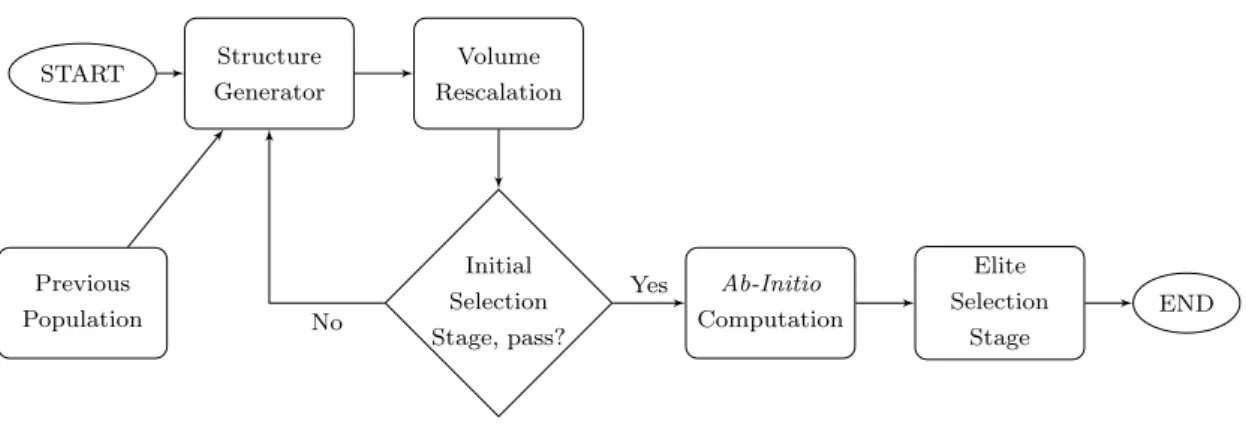
Figure 2: Flowchart of single generation in the method.
Flowchart of single generation of our evolutionary algorithm method is described in Figure 2. This flowchart can be partitioned into two parts; structure generation part and selection and adaptation part.
2.1 Structure Generation
Structure generation plays a keyrole in the evolutionary algorithm method. Structure generation generate a new crystal structure randomly if the cycle is initial generation or from previous gen- eration if it is not initial generation. There are three evolution operators used in this method:
heredity operator, permutation operator, and mutation operator.
Heredity Operator
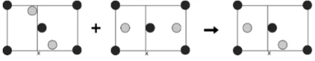
Heredity operator needs two parents to generate an offspring. As described in the previous work [2, 4, 6, 7] and illustrated in Figure 3, first all the parents are transformed arbitrarily. Then the heredity operator chooses a random number between 0.0 to 1.0 to slice one of lattice vectors of the two parents randomly. The plane of this cut is parallel to two other lattice vectors. Then the offspring is constructed by combining atomic position of the two parents delimited by the cut on crystal slab. Lattice parameters of the offspring are weighted average of the two parent’s whose weight is also determined randomly. If the number of atoms in a unit cell is not equal to the parents, the corresponding atom is added or drawn stochastically, so that the number of atoms of the offspring is equal to its parents.
Figure 3: Heredity operator.
Permutation Operator
Permutation operator is a one-parent operator. It needs only one parent to generate an offspring.
As illustrated in Figure 4, it chooses two lattice points of different atomic species and then swap their atomic identity. This procedure is repeated as many as parameter given by the user.
Figure 4: Permutation operator.
The permutation operator explores correct chemical arrangement of the crystal structure in the configurational space [7]. It works only for crystal structure which consists of more than one atomic species. It is completely useless in single species crystals.
Mutation Operator
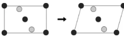
Mutation operator is also a one-parent operator. It distorts lattice vectors of the parent (Figure 5), while atomic coordinates remain unchanged relative to the lattice vectors. This transformation is done using random symmetric matrix [2, 4]. A new lattice vector of the offspring is produced by this following formula:
a0 = (I+)a, (1)
wherea0,aare lattice vectors before and after mutation operation respectively. The (I+) is the symmetric matrix defined as
(I+) =
1 +11 12
2
13
12 2
2 1 +22 23
13 2 2
23
2 1 +33
, (2)
whereij are generated randomly by 0-mean gaussian random distribution between 0.0 and 1.0.
Figure 5: Mutation operator.
2.2 Selection and Adaptation
Each new structure produced by one of the three operators raised above is set to certain volume which is of the best crystal structure of previous generation [7]. This rescalation compensates the pre-condition of the crystal structure generated by the evolution operator which may not be a good initial structure before the crystal structure is relaxed to enhance the structure relaxation in ab-initio computation stage. The volume of initial generation is approximated by atomic radii.
To enhance the structure relaxation more effectively before it is performed, each generated structure must be passed through an initial selection stage. There are three criteria in this selection [2, 4, 6, 7]; minimum interatomic distance, minimum lattice vector length, and minimum and maximum angle of lattice parameters. The structure which violates these criteria is rejected and a new structure is generated again by structure generation using the same operator. This procedure is repeated until it matches to the criteria.
Fitness value of each individual as a function of crystal structure set of varibles is computed in ab-initio computation using first-principle method. Details of the ab-initio method will be described in Section 3.
Elite selection stage plays a role as nature selection of the Lamarckian evolution theory. In this stage, a few worst individuals are discarded and other remaining elite structures are passed to the next cycle of generation and also ranked based on their fitness values. The ranking by the fitness value is useful for procreation or parent selection to generate a new population.
3 Ab-Initio and Simulation Methods
We used density functional theory (DFT) scheme ofab-initiocomputation [8] . Within the scheme, we employed planewave basis function and ultrasoft pseudopotential [9], and used generalized gradient approximation (GGA) for exchange-correlation term [10]. We also used two kinds of k- point meshes used forab-initiocalculation: lowk-point mesh for generating all possible individuals throughout the generations, and highk-point mesh for reoptimization of the last stablest structure of the generations. Our simulation test was carried out on two cases: single phase simulation and phase transition simulation.
3.1 Single Phase Simulation
Single phase simulation was run on silicon (Si) and phosphorus (P). Some details ofab-initio and evolutionary parameters are presented in Table 1.
Table 1: Ab-initioand evolutionary parameters used in single phase simulation.
Parameter Silicon (Si) Phosphorus (P)
Pressure 20 GPa 190 GPa
Energy cut-off wave-function 15 Ry 20 Ry
Energy cut-off density 150 Ry 240 Ry
k-point mesh 4 x 4 x 4 8 x 8 x 8
Number of indiv. per generation 10 10
Probability heredity 0.6 0.7
Probability mutation 0.4 0.3
3.2 Phase Transition Simulation
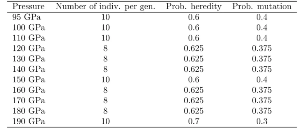
Phase transition simulation was run on phosphorus (P) to see phase transition behavior in high- pressure range using this method. We used several pressure, 95, 100, 110, 120, 130, 140, 150, 160, 170, and 190 GPa. Cut-off energy for wave function and electron density used in this case are 20 Ry and 240 Ry respectively. For generating part of simulation, we used 4 x 4 x 4 k-point mesh. The evolutionary parameters used in this simulation are showed in Table 2. At the end of
Table 2: Evolutionary parameters used in phase transition simulation on phosphorus.
Pressure Number of indiv. per gen. Prob. heredity Prob. mutation
95 GPa 10 0.6 0.4
100 GPa 10 0.6 0.4
110 GPa 10 0.6 0.4
120 GPa 8 0.625 0.375
130 GPa 8 0.625 0.375
140 GPa 8 0.625 0.375
150 GPa 10 0.6 0.4
160 GPa 8 0.625 0.375
170 GPa 8 0.625 0.375
180 GPa 8 0.625 0.375
190 GPa 10 0.7 0.3
simulation, for each different pressure, we then reoptimized the last stablest individual using 16 x 16 x 16k-point mesh to enhance the accuracy of our calculations.
4 Result and Discussion 4.1 Single Phase Simulation
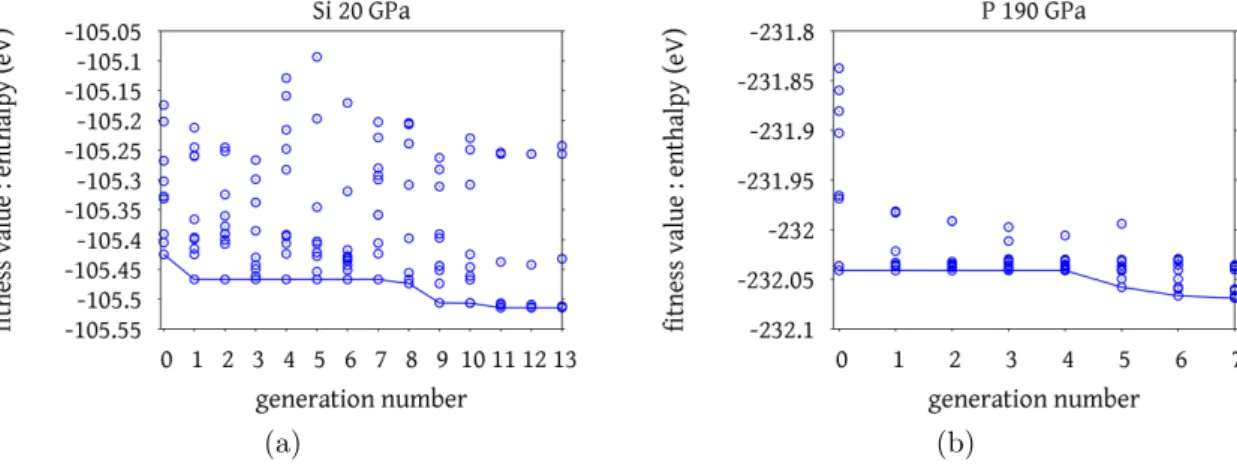
Profiles of silicon and phosphorus in the series of generation are shown in Figure 6. In the profile of silicon, there is a divergent behavior along the fitness value (enthalpy), whereas in phosphorus the enthalpies are converged in the narrow range. Such convergence in the profile may be controlled by the probability of evolution operators. Indeed, in the comparison between two figures, the higher probability of heredity results in the convergence profile on generation series. This convergence is an advantage if one can prevent the same structure to be generated again. However, if one cannot prevent such kind of procedure, this convergence become a disadvantage. It may be effective to prevent redundancy of same structures as Oganovet al. did [6, 11].
(a) (b)
Figure 6: (a) Flow of generation series of silicon at 20 GPa and (b) phosphorus at 190 GPa.
The reoptimized results of the last stablest individual shown in Table 3 give a good agreement with experimental result of the similar materials [12, 13]. Although there is some redundancy of same structures, these resutls show the prediction power of evolutionary algorithm method.
Table 3: Comparison of our result with experimental data.
Lattice Parameters a(˚A) b(˚A) c(˚A) α β γ Vol. (˚A3) Si last generation (20 GPa) 2.471 2.471 2.362 89.978 89.932 115.014 13.071 Si re-optimized (20 GPa) 2.512 2.512 2.380 89.998 89.997 118.293 13.229 Si Experiment [12] (∼16 GPa) 2.551 2.551 2.387 90 90 120 13.45 P last generation (190 GPa) 2.119 2.132 2.047 89.788 90.660 118.955 8.088 P re-optimized (190 GPa) 2.122 2.126 2.045 89.848 90.463 118.986 8.066 P Experiment [13] (151 GPa) 2.175 2.175 2.0628 90 90 120 8.452
4.2 Phase Transition Simulation
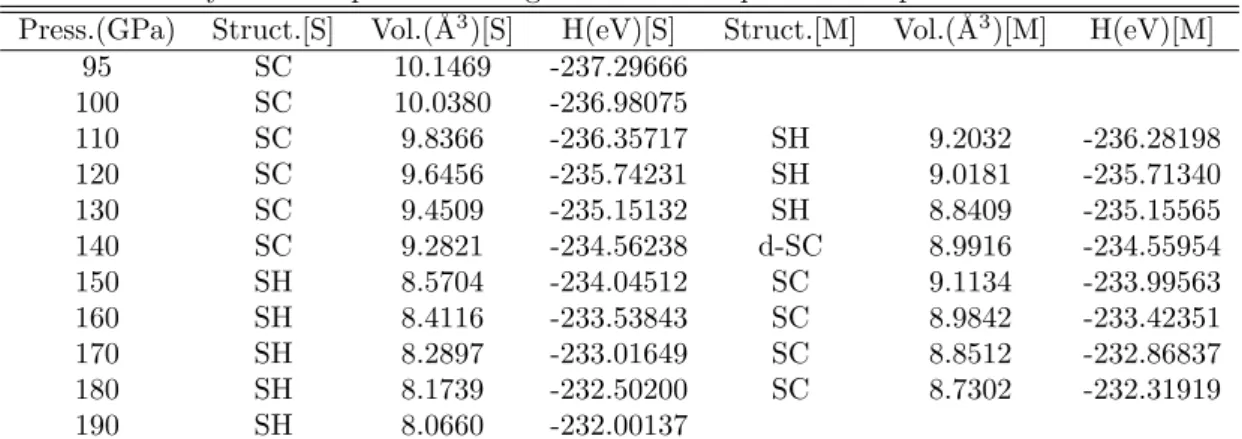
Result of generation series for each pressure is similar to single phase simulation. The reoptimized last stablest generation for all pressures are summarized in Table 4, and we also found metastable structures for some pressures.
Table 4: Summary of the reoptimized last generation of all pressures in phase transition simulation.
Press.(GPa) Struct.[S] Vol.(˚A3)[S] H(eV)[S] Struct.[M] Vol.(˚A3)[M] H(eV)[M]
95 SC 10.1469 -237.29666
100 SC 10.0380 -236.98075
110 SC 9.8366 -236.35717 SH 9.2032 -236.28198
120 SC 9.6456 -235.74231 SH 9.0181 -235.71340
130 SC 9.4509 -235.15132 SH 8.8409 -235.15565
140 SC 9.2821 -234.56238 d-SC 8.9916 -234.55954
150 SH 8.5704 -234.04512 SC 9.1134 -233.99563
160 SH 8.4116 -233.53843 SC 8.9842 -233.42351
170 SH 8.2897 -233.01649 SC 8.8512 -232.86837
180 SH 8.1739 -232.50200 SC 8.7302 -232.31919
190 SH 8.0660 -232.00137
SC = Simple Cubic; SH = simple Hexagonal; d-SC = Distorted Simple Cubic
(a) (b)
Figure 7: Profiles of (a) volume versus pressure and (b) enthalpy versus pressure.
From Table 4, we ploted a graph of volume versus pressure and enthalpy versus pressure, as depicted in Figure 7, with the curve of Murnaghan equation of state in which its parameters are taken from the works of Akahama et al. [13, 14]. It is shown in Figure 7 that the transition pressure obtained from our simulation occurs at around 140 GPa. It is overestimated, compared to the experimental result (137 GPa) of Akahama et al. [13]. Our prediction volumes at the pressures above 150 GPa are also lower than the one predicted by the experiment (Murnaghan state of equation). This underestimation is probably due to thek-point mesh which should be finer
at high-pressure condition or the typical accuracy of GGA approach. The pressure dependences of the volume and enthalpy are consistent with a typical behavior at the first-order phase transition.
Around the transition point, the lattice type is switched over between simple cubic and simple hexagonal structures for both of the ground state structure and the metastable one.
5 Conclusion
We have performed simulations of crystal structure prediction using the evolutionary algorithm method in combination with ab-initio calculation. Results of our simulation have a good agree- ment with the previous experimental works. We found that this implementation of evolutionary algorithm method on crystal structure prediction formed a good new path to answer Maddox’s challenge of the crystal structure prediction. We also found the metastable structure was switched in accordance with the transition pressure. The evolutionary algorithm simulation experienced in this work strongly supports us to the research of crystal structure predictions.
References
[1] J. Maddox. (1988). Crystal from first principles. Nature,335(6187), 210.
[2] G. Trimarchi and A. Zunger. (2007). Global space-group optimization problem: Finding the stablest crystal structure without constraints. Phys. Rev. B,75, 104113-1–104113-8.
[3] P.F. McMillan. (2002). New materials from high-pressure experiments. Nat. Mater., 1(1), 19-25.
[4] A. R. Oganov and C. W. Glass. (2006). Crystal structure prediction using ab initio evolution- ary techniques J. Chem. Phys.,124(24), 244704.
[5] S.M. Woodley, and C.R.A. Catlow. (2009). Structure prediction of titania phases. Computa- tional Materials Science,45(1), 84–95.
[6] A. R. Oganov, Y. Ma, A. O. Lyakhov, M. Valle, and C. Gatti. (2010). Evolutionary crystal structure prediction as a method for the discovery of minerals and materials Reviews in Mineralogy and Geochemistry,71(1), 271–298.
[7] C. W. Glass, A. R. Oganov and N. Hansen. (2006). USPEX-evolutionary crystal structure prediction Computer Physics Communications,175(11-12), 713–720.
[8] P. Hohenberg and W. Kohn. (1964). Inhomogeneous electron gasPhys. Rev.136, B864-B871.;
W. Kohn and L. J. Sham. (1965). Self-consistent equations including exchange and correlation effects Phys. Rev.140, A1133–A1138.
[9] D. Vanderbilt (1990). Soft self-consistent pseudopotentials in a generalized eigenvalue formal- ism Phys. Rev. B,41, 7892-7895.
[10] J. P. Perdew, J. A. Chevary, M. R. Pederson, D. J. Singh, and C. Fiolhais. (1992). Atoms, molecules, solids, and surfaces: Applications of the generalized gradient approximation for exchange and correlation, Phys. Rev. B,46, 6671-6687.
[11] A.R. Oganov and M. Valle. (2009). How to quantify energy landscapes of solids. J. Chem.
Phys.,130(10), 104504.
[12] J. Z. Hu, L. D. Merkle, C. S. Menoni, and I. L. Spain. (1986). Crystal data for high-pressure phases of silicon Phys. Rev. B,34(7), 4679.
[13] Y. Akahama, M. Kobayashi, and H. Kawamura. (1999). Simple-cubic-simple-hexagonal tran- sition in phosphorus under pressure. Phys. Rev. B,59(13), 8520–8525.
[14] Y. Akahama, H. Kawamura, S. Carlson, T. L. Bihan, and D. H¨ausermann. (2000). Structural stability and equation of state of simple-hexagonal phosphorus to 280 GPa: Phase transition at 262 GPa. Phys. Rev. B,61(5), 3139–3142.