Hamilton Cycles, Paths and Spanning Trees in a Graph

(1)

Hamilton Cycles, Paths and Spanning Trees in a Graph

March 2009

Kenta Ozeki

(2)

Acknowledgments

I am grateful to all people who contributed to this thesis.

First of all, I would like to express my deep gratitude to Professor Katsuhiro Ota, for his suggestions, encouragement, careful reading and so on. Without his advice and help, this thesis would not complete. Also I thank Professor Yoshiaki Oda for his valuable advice and kindness.

I am grateful to Professor Tomoki Yamashita, who gave me a chance to study cycles, paths and trees, for some joint work and fruitful discussions. I would like to thank Professor Hikoe Enomoto, Professor Mikio Kano, and Professor Akira Saito, for some helpful suggestions and joint work. I would like to thank to Pro- fessor Kiyoshi Yoshimoto, Professor Haruhide Matsuda, and Professor Ken-ichi Kawarabayashi for the valuable discussions and some joint work. Also thanks to all members of Ota–Oda Laboratory at Keio University, Graph Seminar at Tokyo Uni- versity of Science, and Topological Graph Theory Seminar at Yokohama National University for their helpful comments and encouragement.

Finally, I thank my family and all of my friends. They have been a great support to me.

Kenta Ozeki 2009

(3)

Preface

This thesis is written on the subject “Hamilton cycles, paths and spanning trees in a graph.” The basis of this thesis is formed by papers written during these four years.

After an introductory chapter, the reader will ﬁnd ten chapters. General terminology of Graph Theory is found in Chapter 2. The other chapters can be read independently from one another. The main part of this thesis is divided into two parts; the ﬁrst one is some relaxed structures of a hamilton cycle, another is spanning trees as a relaxation of a hamilton path.

A cycle in a graph is called a hamilton cycle if it passes all vertices of the graph.

A problem of determining whether a given graph has a hamilton cycle or not is important in Graph Theory, but it is known as a “difficult” one in a Combinatorial sense. Therefore we do not deal with this problem directly, and consider from the following two aspects; to find better sufficient conditions for the existence of a hamilton cycle, and to study relaxed structures of a hamilton cycle. In this thesis, we focus on the second aspect, in particular, we consider degree sum conditions and independence number conditions for the existence of such structures.

A hamilton cycle must pass all vertices of a graph. Relaxing this property of a hamilton cycle, we consider a cycle passing all specified vertices. We shall give a sufficient condition for the existence of such a cycle in terms of degrees and independent sets of specified vertices. Moreover, a cycle passing not only specified vertices but also specified edges has been studied. We discuss about these cycles in Chapters 3 and 5, respectively.

As another notion of relaxing a hamilton cycle, we considera dominating cycle.

A cycle is called dominating if removing all vertices of it results in a graph with no edges. Deﬁnitely, a hamilton cycle is dominating, but the converse does not generally hold. We sometimes consider a dominating cycle as “close” to a hamilton cycle, because the outside of the cycle must be small. Moreover, it is known that a dominating cycle has some good properties as a hamilton cycle. Therefore many researchers have studied a dominating cycle. We focus on a dominating cycle in Chapter 4. In Chapter 6, we introduce an invariant “Relative Length,” which concerns with a property of a dominating cycle. We mention the relationship between

(4)

a dominating cycle or “Relative Length” and the length of a longest cycle of a graph in Chapter 7.

Ahamilton path of a graph is a path passing all vertices. Similarly to a hamilton cycle, it is known that a problem of determining whether a given graph has a hamilton path or not is a “diﬃcult” one. Therefore we are also interested in some relaxed concept of a hamilton path, like a hamilton cycle. The rest ﬁve chapters deal with spanning trees with particular properties which are relaxed concepts of a hamilton path.

The most important one is a spanning tree whose maximum degree is at mostk, called a spanning k-tree. It appears in Chapters 8–10. In particular, we will focus on ak-tree containing speciﬁed vertices in Chapter 8, a spanningf-tree, in Chapter 9, and the concept “prism hamiltonian” in Chapter 10, respectively.

In the remaining two chapters, we will study other directions of relaxed structures of a hamilton path; a spanning tree with bounded number of vertices of degrees one, or with bounded number of vertices of degrees at least three. We focus on these spanning trees in Chapters 11 and 12, respectively.

(5)

10.1 Relationship to k-trees and k-walks . . . . 149 10.2 Prism hamiltonicity of particular classes . . . 150 10.3 Degree conditions for prism hamiltonicity . . . 152 11 Spanning trees with bounded number of leaves 157 11.1 On general graphs . . . 157 11.2 On claw-free graphs . . . 158 12 Spanning trees with bounded number of branch vertices 169 12.1 On general graphs and bipartite graphs . . . 169 12.2 On claw-free graphs . . . 171

References 176

(7)

Chapter 1 Introduction

In this thesis, we deal with cycles, paths and trees with some properties related to a hamilton cycle or a hamilton path. A hamilton cycle is a cycle passing through all vertices of a graph. We call a graph having a hamilton cyclehamiltonian. Similarly, a hamilton path is a path passing through all vertices of a graph. An interest of a hamilton cycle originates in the relationship to Four Color Problem, but recently, it concerns with many other topics or areas. So study on a hamilton cycle is one of the most important and basic topics in Graph Theory.

One of the huge targets of this study is to find a necessary and sufficient condition for the existence of a hamilton cycle, except for a trivial one. However, in contrast with an Eulerian circuit, it seems to be difficult and no one have succeeded. In fact, the problem of determining whether a given graph has a hamilton cycle or not belongs to the class of N P-complete problems, that is, a difficult problem in a Combinatorial sense. So we have focused on sufficient conditions or some relaxed structures of a hamilton cycle. There are many sufficient conditions for the existence of a hamilton cycle. The following is a classical result on it.

Theorem 1.1 (Dirac [41]) Let G be a graph of order n ≥ 3. If the minimum degree is at least ¹₂n, then G has a hamilton cycle.

To satisfy the assumption of Theorem 1.1, “all vertices” of a graph must have high degrees. However, this condition is too strong in a sense. Ore considered that even if some vertices have low degrees, if all of them are adjacent each other, then the graph might have a hamilton cycle. Actually, he showed the following theorem.

When the required number of nonadjacent vertices cannot be taken, we deﬁne the value of “the minimum degree sum” as +∞.

Theorem 1.2 (Ore [130]) Let G be a graph of order n ≥ 3. If the minimum degree sum of two nonadjacent vertices is at least n, thenG has a hamilton cycle.

As a condition other than the degrees, Chv´atal and Erd˝os considered the one

(8)

concerning the independence number and the connectivity of a graph. We denote the independence number and the connectivity of a graph G by α(G) and κ(G), respectively. Note that it is known that Theorem 1.3 implies Theorem 1.2.

Theorem 1.3 (Chv´atal and Erd˝os [37]) LetGbe a2-connected graph. Ifα(G) is at most κ(G), thenG has a hamilton cycle.

Starting from Theorems 1.1–1.3, many researchers have considered the conditions concerning with the degrees or the independence number and the connectivity.

A hamilton cycle must pass through “all vertices” of a graph. In this sense, we can consider a relaxation of the concept of a hamilton cycle; a cycle passing through all “specified vertices.” A set of specified vertices is called cyclable in a graph G if G has a cycle passing through all of them. In order to guarantee the existence of a hamilton cycle, we consider a degree condition or an independence number condition of all vertices as in Theorems 1.1–1.3. However when we would like to show the cyclability of specified vertices, it is not necessary to deal with the degrees or the independence number of all vertices. In fact, it often suffices to consider only that of the specified vertices as follows. For a vertex set S, we denote the independence number and the connectivity ofS byα(S) andκ(S), respectively.

(See Chapter 3).

Theorem 1.4 (Shi [149]) Let G be a 2-connected graph of order n, and S ⊆ V(G). If the minimum degree sum of pairwise nonadjacent vertices inS is at least n, thenS is cyclable in G.

Theorem 1.5 ([135]) Let G be a 2-connected graph, and S ⊆ V(G). If α(S) is at mostκ(S), then S is cyclable in G.

Motivated by the improvement of Theorem 1.1 to Theorem 1.2, Bauer, Broersma, Li and Veldman [13] considered a condition of degree sum of three vertices for the existence of a hamilton cycle. Recently, this result was extended to the result on cyclability by Broersma, H. Li, J. Li, Tian and Veldman.

Theorem 1.6 (Broersma, H. Li, J. Li, Tian and Veldman [30]) LetGbe a graph of order n, and S ⊆ V(G) with κ(S) ≥ 2. If the minimum degree sum of three pairwise nonadjacent vertices of S is at least n+κ(S), then S is cyclable in G.

Again, motivated by the improvement of the condition of degree sum of two vertices in Theorem 1.4 to three vertices in Theorem 1.6, we show the following result on the degree sum of four vertices. In Chapter 3, we focus on a hamilton cycle and cyclability of speciﬁed vertices, and gave the proof of Theorem 1.7.

(9)

Theorem 1.7 ([135]) LetGbe a graph of ordern, andS ⊆V(G)with κ(S)≥3.

If the minimum degree sum of four pairwise nonadjacent vertices in S is at least n+κ(S) +α(S)−1, then S is cyclable in G.

Recently, Ota gave a result by a condition on the degree sum of more vertices.

But Theorems 1.6 and 1.7 cannot be implied by Theorem 1.8. In fact, there exist some examples showing the above fact and we will show them in Chapter 3.

Theorem 1.8 (Ota [132]) Let G be a graph of order n, and S ⊆ V(G) with κ(S)≥2. If, for any t≥κ(S), the minimum degree sum of t+ 1pairwise nonadja- cent vertices in S is at least n+t²−t, then S is cyclable in G.

Along the above stream, many suﬃcient conditions on a hamilton cycle or cyclability of speciﬁed vertices have been found. On the other hand, as other approach to a hamilton property, many relaxations of hamilton cycles are also considered.

One of the most important relaxations is the concept of a dominating cycle. A cycle C in a graph G is called dominating if at least one end-vertex of any edge of Gis contained inC. By the deﬁnitions, a hamilton cycle is also a dominating cycle but generally the converse does not hold. A dominating cycle has considered as a

“pre-hamilton” cycle. This is because, in order to find a hamilton cycle in a given graph, sometimes we first try to find a dominating cycle before it. For example, if some longest cycle in G is dominating and the independence number of G is at most the minimum degree, then G has a hamilton cycle.

Recently, the concept of dominating cycles becomes more important because of not only the meaning of a “pre-hamilton cycle” but also the relationship with other properties, for example, circumference of a graph (the length of a longest cycle).

We will mention this relationship in Chapter 7. Therefore we are interested in the concept of dominating cycles itself. In 1980, Bondy showed the following result, which is a generalization of Nash-Williams’ result [127]. This is a basic result on dominating cycles using a degree sum condition.

Theorem 1.9 (Bondy [26]) LetG be a2-connected graph of order n≥3. If the minimum degree sum of three pairwise nonadjacent vertices is at least n+ 2, then each longest cycle in G is dominating.

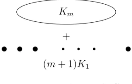
As well as degree conditions, one might expect an independence number condition on dominating cycles. However, considering the graph G₁ =K_k+ (k + 1)K_m with m≥2, in a sense, it fails for general graphs. Since α(G₁) =k+ 1 =κ(G₁) + 1 and G₁ has no dominating cycle, even if we would like to ﬁnd a dominating cycle by an independence number condition, the same condition that “α(G) is at most κ(G)” as Theorem 1.3 is needed. Motivated by the above reason, when we consider an independence number condition for a dominating cycle, it is necessary to restrict

(10)

ourselves to some particular classes of graphs, at least we must avoid some graphs like G₁. Enomoto, Kaneko, Saito and Wei considered a class of triangle-free graphs and gave an independence number condition for a dominating cycle.

Theorem 1.10 (Enomoto, Kaneko, Saito and Wei [48]) Let G be a2-connected triangle-free graph. If α(G) is at most 2κ(G)−2, then every longest cycle in G is dominating.

It is unknown whether the condition of Theorem 1.10 is sharp or not. But there exists a triangle-free graph G with α(G) is equal to 2κ(G) such that any longest cycle of G is not dominating. In Chapter 4, we discuss some results on a dominating cycle and show the following theorem. By the above example, the condition of Theorem 1.11 is best possible.

Theorem 1.11 ([136]) Let G be a 2-connected triangle-free graph. If α(G) is at most 2κ(G)−1, then there exists a longest cycle in G which is dominating.

Similarly to a cycle passing through “specified vertices,” sometimes we consider cycles passing through not only “specified vertices,” but also “specified edges.” Of course there exist some edges that cannot be passed by one cycle. When specified edges induce a graph having a vertex of degree at least three, it is trivially impossible to find a cycle passing through all such edges. So, as those specified vertices and edges, we consider a linear forest, that is a forest such that each component of it is a path (possibly it may consist of only one vertex).

In Chapter 5, we consider a cycle passing through speciﬁed edges. In particular, we concentrate on a dominating cycle and a hamilton cycle passing through a given linear forest. The following is the one for a dominating cycle. When we take a linear forestF with E(F) =∅ and|V(F)| ≤3, the condition of Theorem 1.12 is identical to that of Theorem 1.9. Thus, Theorems 1.12 is a generalization of Theorem 1.9.

Note that Theorem 1.12 does not guarantee the existence of a cycle passing through a given linear forest, however, H¨aggkvist and Thomassen [81] showed that such a cycle exists if the graph is (m+r)-connected.

Theorem 1.12 ([137]) Let G be an (m+ 2)-connected graph of order n. Let F be a linear forest with |E(F)|=m and letr be the number of the isolated vertices of F. If the minimum degree sum of three pairwise nonadjacent vertices is at least n+2m+max{r−1,2}, then every longest cycleC passing throughF is dominating.

On the other hand, some suﬃcient conditions for the existence of a hamilton cycle have been also considered. P´osa showed the following theorem as a generalization of Theorem 1.2; for a graph Gof order n≥3 and for a linear forestF with

|E(F)|=m, if the minimum degree sum of nonadjacent vertices is at leastn+m, then Ghas a hamilton cycle passing throughF. In Chapter 5, we show some other

(11)

suﬃcient conditions for the existence of a hamilton cycle through a given linear forest. One of them is the following. When m = 0 in Theorem 1.13, it is identical to Theorem 1.6 for the case whereS =V(G). Thus, Theorem 1.13 is a generalization of Theorem 1.6, in a sense. We will survey on a cycle passing through given edges and show Theorems 1.12 and 1.13 in Chapter 5.

Theorem 1.13 ([137]) LetGbe an(m+ 2)-connected graph of ordern, andF be a linear forest with|E(F)|=m. Suppose thatn ≥2κ(G) + 2m+ 1. If the minimum degree sum of three pairwise nonadjacent vertices is at least n+κ(G) +m, thenG contains a hamilton cycle passing through F.

Recently, a new invariant, called relative length, is also considered. Now we denote the order (the number of vertices) of a longest path and a longest cycle of a graph G by p(G) and c(G), respectively. The relative length of a graph G, denoted by diff(G), is defined as the difference between these two invariants, that is, diff(G) :=p(G)−c(G). The relative length looks strange and complex, however, it is useful and has some good applications. It is easy to see that for a connected graph G, diff(G) = 0 if and only ifGis hamiltonian and if diff(G)≤1, any longest cycle of Gis dominating.

In addition to above, more cycle-related properties are implied by the low relative length. For example, it is shown in [111] that for a graph G with diﬀ(G) ≤ 1, the circumference ofGis at least min{n+δ−α(G), n}, and in [134], for a graphGwith diﬀ(G)≤2, the circumference ofG is at least min{n+ 2δ−2α(G)−2, n}, where δ be the minimum degree of G. As in Chapter 6, more properties are implied by the low relative length.

As mentioned before, a dominating cycle is regarded as a “pre-hamilton” cycle.

Since any longest cycle of G is dominating if diff(G) ≤ 1, the property diff(G) ≤ 1 can be also regarded as the property “pre-hamiltonian.” Moreover, not only diff(G)≤ 1, but also the low relative length, diff(G) ≤2 or something else, seems to have such property. In fact, by the above result on the circumference, for a graph G with diff(G)≤2, ifα(G) + 1 is at most the minimum degree of G, thenG has a hamilton cycle.

Relative length was ﬁrst posed by Enomoto, van den Heuvel, Kaneko and Saito in 1995. In the same paper, they gave a degree sum condition for a graph G to satisfy diﬀ(G)≤1. Note that this result is stronger than Theorem 1.9.

Theorem 1.14 (Enomoto, van den Heuvel, Kaneko and Saito [46]) Let G be a 2-connected graph of order n. If the minimum degree sum of three pairwise nonadjacent vertices is at least n+ 2, then diﬀ(G)≤1.

In [111], Li, Saito and Schelp considered the relationship between the property

“diﬀ(G) ≤1” and a minimum degree sum of four vertices condition. They proved

(12)

that for a 3-connected graph G of order n, if the minimum degree sum of four pairwise nonadjacent vertices is at least ³₂n+1, then diﬀ(G)≤1 and also conjectured that the sharp coeﬃcient of n is ⁴₃. Lu, Liu and Tian gave a sharp bound on the condition.

Theorem 1.15 (Lu, Liu and Tian [118]) Let G be a 3-connected graph of or- der n. If the minimum degree sum of four pairwise nonadjacent vertices is at least

13(4n+ 5), then diﬀ(G)≤1.

In Chapter 6, we prove the following result on diﬀ(G)≤2. Moreover, we show some applications of relative length and give some other results on the low relative length.

Theorem 1.16 ([134]) LetGbe a 3-connected graph of order n. If the minimum degree sum of four pairwise nonadjacent vertices is at least n+ 6, thendiﬀ(G)≤2.

We sometimes regard a graph with a hamilton path as having a good property.

So we often try to ﬁnd suﬃcient conditions for a graph without a hamilton path to have the low relative length. In [46], Enomoto, van den Heuvel, Kaneko and Saito gave a degree sum of three vertices condition of it.

Theorem 1.17 (Enomoto, van den Heuvel, Kaneko and Saito [46]) Let G be a connected graph of order n. If the minimum degree sum of three pairwise nonadjacent vertices is at leastn, then eitherdiﬀ(G)≤1orGhas a hamilton path.

Theorems 1.14 and 1.17 suggest that the connectivity and degree sum condition can be weakened for graphs without a hamilton path. Therefore, one might expect that the conditions of other results on the low relative length can be also weakened for graphs without a hamilton path. By the expectation of Theorem 1.15, we prove the following result.

Theorem 1.18 ([99]) Let G be a 2-connected graph of order n. If the minimum degree sum of four pairwise nonadjacent vertices is at least ¹₃(4n−2), then either diﬀ(G)≤1 or Ghas a hamilton path.

On the other hand, in 2002, Schiermeyer and Tewes [148] investigated the re- lation between a minimum degree sum of three vertices and diﬀ(G) ≤ 2 in a 2- connected graph G. A path P of a graphGis said to be dominating if the removal of all vertices of P from G results in a graph with no edge. They showed that for a 2-connected graph G of order n, if the minimum degree sum of four pairwise nonadjacent vertices is at leastn+ 3, then either diﬀ(G)≤2 or every longest path inGis dominating. However, considering the relations between Theorems 1.14 and 1.17 and between Theorems 1.15 and 1.18, the conclusion of the above result seems

(13)

to be weak. The following theorem is one improvement of Schiermeyer and Tewes result.

Theorem 1.19 ([99]) Let G be a 2-connected graph of order n. If the minimum degree sum of four pairwise nonadjacent vertices is at least n + 3, then either diﬀ(G)≤2 or Ghas a hamilton path.

We also give proofs of Theorems 1.18 and 1.19 in Chapter 6.

If a graph G has a long cycle (for example, comparing the order of G), we can regard G as a graph being “close” to hamiltonian. So we are interested in the circumference c(G), that is the order of a longest cycle. Many researchers have been established the lower bound of the circumference by various invariants. We will survey those of the circumference in Chapter 7. The following results concerns with the circumference and the minimum degree sum of three vertices or p(G).

Theorem 1.20 (Fournier and Fraisse [64]) Let G be a 2-connected graph of order n. Then c(G)≥min{2d/3, n}, where d is the minimum degree sum of three pairwise nonadjacent vertices.

Theorem 1.21 (Bondy and Locke [28]) Let G be a 3-connected graph. Then c(G)≥2(p(G)−1)/5.

In Chapter 7, we show the following result, which shows that the bounds of Theorems 1.20 and 1.21 can be improved by considering the minimum degree sum of three vertices and p(G) at the same time.

Theorem 1.22 ([138]) Let G be a 3-connected graph. Then c(G) ≥ min{d− 3, p(G)−1}, where d is the minimum degree sum of three pairwise nonadjacent vertices.

In other words, for any 3-connected graph G, c(G)≥d−3 or diﬀ(G)≤1. This is an improvement of a result by Fraisse and Jung [66], which says that for any 3-connected graph G, c(G) ≥ d −3 or any longest cycle in G is dominating. In Chapter 7, we will introduce some results on the circumference and prove Theorem 1.22

As mentioned above, we have considered the relaxation of the concept of a hamilton cycle, for example, a cycle containing speciﬁed vertices, dominating cycles, relative length and the circumference. In the rest of introduction of this thesis, we deal with relaxations of the concept of a hamilton path. The most important relaxation of it is aspanning k-tree. A k-tree is a tree whose maximum degree is at most k. Deﬁnitely a spanning 2-tree is equivalent to a hamilton path.

(14)

As immediate corollaries of Theorems 1.2 and 1.3, for a connected graph G of order n, we obtain the following result; If the minimum degree sum of nonadjacent vertices is at least n−1 or ifα(G) is at mostκ(G) + 1, thenGhas a hamilton path.

Win, and Neumann-Lara and Rivera-Campo extended those corollaries, and gave a degree sum condition and an independence number condition to have a spanning k-tree, respectively.

Theorem 1.23 (Win [168]) Let k be an integer with k ≥ 2, and let G be a connected graph of order n. If the minimum degree sum of k pairwise nonadjacent vertices is at least n−1, then Ghas a spanning k-tree.

Theorem 1.24 (Neumann-Lara and Rivera-Campo [128]) Letk be an inte- ger withk ≥2, and letGbe anm-connected graph. Ifα(G)is at most(k−1)m+ 1, then G has a spanning k-tree.

Similarly to dealing with a cycle containing speciﬁed vertices as a relaxation of the concept of a hamilton cycle, it is natural to consider ak-tree containing speciﬁed vertices. Motivated by such a consideration, Matsuda and Matsumura proved the following theorem.

Theorem 1.25 (Matsuda and Matsumura [121]) LetGbe a connected graph of ordernand letS ⊆V(G). If the minimum degree sum ofk pairwise nonadjacent vertices in S is at least n−1, then G has ak-tree containing all vertex in S.

For a connected graph G and S ⊆ V(G), if α(S) is at most k − 1, then G and S trivially satisfy the assumption of Theorem 1.25, and hence it has a k- tree containing S. So Theorem 1.25 also gave an independence number condition.

However, comparing Theorem 1.24, the condition “α(S) is at most k−1” seems too strong for a graph G to have a k-tree containing S. In addition, although the degree sum bound of Theorem 1.25 is best possible, we may be able to decrease it if a graph has high connectivity. Motivated by these consideration, we show the following result, which is a k-tree analogy of Theorem 1.8. In Chapter 8, we will give a proof of Theorem 1.26

Theorem 1.26 ([36]) Let k be an integer with k ≥ 3 and let G be a graph of order n. Let S ⊆ V(G) with κ(S) ≥ 1. If for every l ≥ κ(S), the minimum degree sum of t pairwise nonadjacent vertices in S is at least n+tl−kl−1, where t= (k−1)l+ 2− ^l⁻¹_k , thenG has a k-tree containingS.

We may consider a more general concept than a spanning k-tree. Let G be a graph and let f be a mapping from V(G) to positive integers. A tree T of G is called anf-tree if for anyx∈V(T), the degree ofxinT is at mostf(x). Deﬁnitely, when f is a constant mapping taking value k, an f-tree is equivalent to a k-tree.

(15)

Matsuda and Matsumura gave a result on the existence of a spanning k-tree with speciﬁed leaves, which is an extension of Theorem 1.24.

Theorem 1.27 (Matsuda and Matsumura [120]) Let m, k and s be integers with k ≥2, 0≤s≤k and s+ 1≤m and letG be an m-connected graph. If α(G) is at most(m−s)(k−1) + 1, then for any svertices of G, Ghas a spanningk-tree T such that the s speciﬁed vertices are contained in the set of leaves.

Extending this result to a spanningf-tree, the following conjecture is proposed.

Conjecture 1.28 ([49]) Let m be an integer, G be an m-connected graph and f be a mapping fromV(G)to positive integers. If

x∈V(G)f(x)≥2(|V(G)| −1) and α(G)is at mostmin _x_∈_R(f(x)−1) :R⊆V(G),|R|=m

+ 1, then there exists a spanning f-tree.

Suppose that there exists a spanning f-tree T. Then

x∈V(G)

f(x) ≥

x∈V(G)

dT(x)

= 2|E(T)|

= 2(|V(G)| −1).

Therefore for the existence of a spanning f-tree, the condition “

x∈V(G)f(x) ≥ 2(|V(G)| −1)” is a trivial necessary condition. Note that the independence number condition of Conjecture 1.28 is best possible if it is true.

In Chapter 9, we show the following result, which gives a partial solution to Conjecture 1.28. For a mapping f, let Si(f) := {x ∈ V(G) : f(x) = i} and s_i(f) :=|S_i(f)|.

Theorem 1.29 ([49]) Letmbe a positive integer,Gbe anm-connected graph and f be a mapping from V(G) to positive integers. Suppose s₁(f) +s₂(f) ≤ m+ 1,

x∈V(G)f(x) ≥ 2(|V(G)| −1) and α(G) is at most min _x_∈_R(f(x)−1) : R ⊆ V(G),|R|=m

+ 1. Then there exists a spanning f-tree in G.

Letf₁ be a mapping onV(G) which assigns 1 tos given vertices andk to other vertices. Then a spanning f₁-tree is a spanning k-tree satisfying the conclusion of Theorem 1.27. Moreover,

min

x∈R

(f₁(x)−1) :R⊆V(G),|R|=m

+ 1

= s(1−1) + (m−s)(k−1) + 1

= (m−s)(k−1) + 1,

and hence Theorem 1.27 is a special case of Conjecture 1.28. Ifk≥3, thens₁(f₁) + s₂(f₁) =s ≤m+ 1. This implies that Theorem 1.29 is a generalization of Theorem

(16)

1.27 for k ≥ 3. Note that essential part of the proof of Theorem 1.27 is only the case k ≥ 3, because the case k = 2 is contained in results on a hamilton path like Theorem 1.3.

Again we consider a spanning k-tree as a relaxation of a hamilton path, that is, a spanning tree with maximum degree at mostk. Similarly to this consideration for a hamilton cycle, the concept of a spanning k-walk has been considered. A k-walk is a closed walk that passes through each vertex at most k times. It is clear that a spanning 1-walk is equivalent to a hamilton cycle, so in this sense, a spanning k-walk is a relaxed concept of it. It is known that the existence of a spanning k- tree implies that of a spanningk-walk, and that the existence of a spanningk-walk implies that of a spanning (k+ 1)-tree. Thus, the properties “having a spanning k-tree” and “having a spanningk-walk” provide a hierarchy for measuring how far a graph is from being hamiltonian.

The prism over G is deﬁned as the Cartesian product of the graphs G and K₂. Formally, it consists of two copies of G and a matching joining the corresponding vertices. A graphGis called prism hamiltonian if the prism overG has a hamilton cycle. The property of “being prism hamiltonian” is between the properties “having a spanning 2-tree” and “having a spanning 2-walk,” that is, if G has a spanning 2-tree then G is prism hamiltonian, and if G is prism hamiltonian then G has a spanning 2-walk. Therefore, the property of “being prism hamiltonian” can be added to the above “k-tree and k-walk” hierarchy.

As mentioned in Theorem 1.23, Win gave a sharp degree sum of k vertices condition for a connected graph G to have a spanning k-tree. For a spanning k- walk, Jackson and Wormald prove the following result.

Theorem 1.30 (Jackson and Wormald [92]) Let G be a connected graph of order n, and let k be an integer with k ≥ 1. If the minimum degree sum of k+ 1 vertices which are pairwise nonadjacent is at leastn, thenGhas a spanningk-walk.

By Theorems 1.23 and 1.30 for a connected graphG of ordern, if the minimum degree sum of nonadjacent vertices is at least n−1, then G has a spanning 2-tree (a hamilton path), and if the minimum degree sum of three pairwise nonadjacent vertices is at least n, then G has a spanning 2-walk. Since the property of “being prism hamiltonian” is between “having a spanning 2-tree” and “having a spanning 2-walk,” it is natural to pose the following problem; Determine a sharp degree sum condition for connected graphs to be prism hamiltonian. As an answer to this problem, in Chapter 10, we show the following result.

Theorem 1.31 ([133]) Let G be a connected graph of order n. If the minimum degree sum of three pairwise nonadjacent vertices is at least n, then G is prism

(17)

hamiltonian.

Therefore for a connected graph G of order n, if the minimum degree sum of three pairwise nonadjacent vertices is at leastn,Ghas not only the property “having a spanning 2-walk” but also “being prism hamiltonian.” Moreover, there exists a graph showing that the degree sum condition of Theorem 1.31 is best possible. In this sense, the property of “being prism hamiltonian” seems closer to the property

“having a 2-walk” than “having a spanning 2-tree.”

We have considered a spanning tree with bounded degrees as a relaxation of the concept of a hamilton path. But there are some other relaxations of it. In the rest of introduction of this thesis, we concentrate on them, in particular, the following two concepts of spanning trees.

We can regard a hamilton path as a spanning tree such that exactly two vertices have the degree one and others have the degree two. In this sense, a spanning tree with bounded number of vertices of degree one or with bounded number of vertices of degree at least three is a relaxation of the concept of a hamilton path. A vertex in a spanning tree of degree one (at least three) is called a leaf (a branch vertex, respectively.) Notice that a hamilton path is a spanning tree with exactly two leaves and no branch vertices. In Chapters 11 and 12, we consider a spanning tree with bounded number of leaves and branch vertices, respectively.

This study is also based on the immediate corollaries of Theorems 1.2 and 1.3; for a graphGof order n, if the minimum degree sum of nonadjacent vertices is at least n−1 or ifα(G) is at mostκ(G)+1, thenGhas a hamilton path. In other words, such graph has a spanning tree with exactly two leaves and no branch vertices. Broersma and Tuinstra extended the result for a spanning tree with bounded number of leaves.

Theorem 1.32 (Broersma and Tuinstra [31]) Letk ≥2be an integer and let Gbe a connected graph of ordern ≥2. If the minimum degree sum of nonadjacent vertices is at least n−k+ 1, then G has a spanning tree with at most k leaves.

The case k= 2 guarantees the existence of a hamilton path, which is the equivalent to a corollary of Theorem 1.2, so Theorem 1.32 contains it. Note that the graph K_m+ (m+k)K₁ shows the best possibility of Theorem 1.32. Although the degree condition of Theorem 1.32 is sharp, we may decrease it by restricting ourselves to some special classes of graphs. Of course, such classes have to avoid graphs like K_m+ (m+k)K₁.

One of the important classes having the above property is a class of claw-free graphs. A claw is a graph isomorphic to K₁_,₃, that is a complete bipartite graph with partite sets of order one and three, respectively. A graph is calledclaw-free if it has no induced claw. Since a claw-free graph has several interesting properties and

(18)

relationship to some problems of Graph Theory, many researchers have considered about a class of claw-free graphs. In fact, Matthews and Sumner proved that the degree condition of Theorem 1.1 can be decreased if we restrict ourselves to claw-free graphs.

Theorem 1.33 (Matthews and Sumner [123]) Let G be a 2-connected claw- free graph of order n. If the minimum degree if at least (n−2)/3, then G has a hamilton cycle.

Therefore, in view of Theorem 1.33, for claw-free graphs, a much weaker condition may yield the same conclusion as in results for other structures. Motivated by this observation, we study a degree sum condition for a claw-free graph to have a spanning tree with a bounded number of leaves, and give the following theorem.

Theorem 1.34 ([96]) Letk ≥2be an integer and let Gbe a connected claw-free graph of order n. If the minimum degree sum of k+ 1 nonadjacent vertices is at least n−k, then G has a spanning tree with at mostk leaves.

In Chapter 11, we concentrate on a spanning tree with bounded number of leaves.

On the other hand, in Chapter 12, we consider a spanning tree with bounded number of branch vertices. Gargano, Hammar, Hell, Stacho and Vaccaroa gave a degree sum condition for claw-free graphs to have a spanning tree with bounded number of branch vertices.

Theorem 1.35 (Gargano, Hammar, Hell, Stacho and Vaccaroa [72]) Lets≥ 0be an integer and letGbe a connected claw-free graph of ordern. If the minimum degree sum ofs+ 3nonadjacent vertices is at leastn−s−2, thenGhas a spanning tree with at most s branch vertices.

Note that it is unknown whether the condition of Theorem 1.35 is sharp or not. Theorem 1.35 also implies an independence number condition; for a connected claw-free graphG, ifα(G) is at mosts+ 2, thenGhas a spanning tree with at most s branch vertices. However, this condition is not best possible. In fact, we obtain the following result.

Theorem 1.36 ([122]) Lets ≥0be an integer and letGbe a connected claw-free graph. Ifα(G) is at most2s+ 2, then Ghas a spanning tree with at mosts branch vertices.

By Theorem 1.36, we can ﬁnd 2s+ 3 pairwise nonadjacent vertices in G if we assume thatGhas no spanning tree with at mostsbranch vertices. In this sense, we

(19)

conjecture a weaker condition than Theorem 1.35 can also guarantee the existence of a spanning tree with bounded number of branch vertices as follows;

Conjecture 1.37 ([122]) Lets ≥0 be an integer and let G be a connected claw- free graph of order n. If the minimum degree sum of2s+ 3nonadjacent vertices is at least n−2, thenG has a spanning tree with at most s branch vertices.

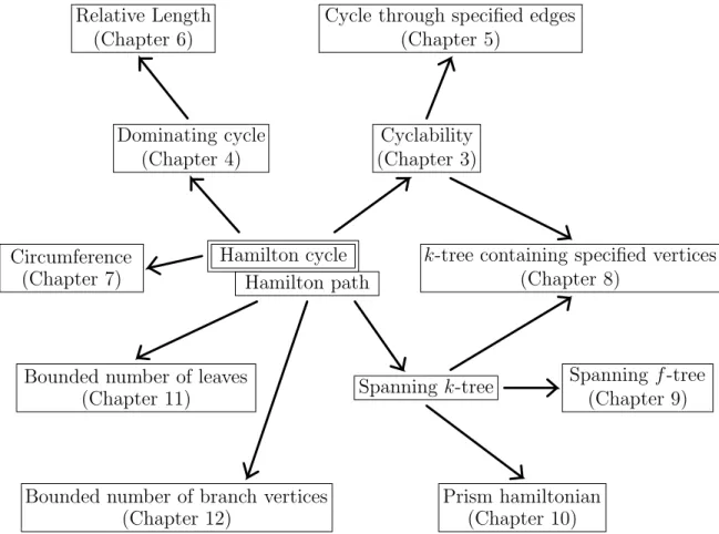
In the last of Introduction, we show the relationship between the relaxed structures of (or invariants concerning with) hamilton cycles or hamilton paths considered in each Chapters 3–12 of this thesis. (See Figure 1.1.) An arrow from A to B means that B is an extended structure (or a generalized invariant) of A.

Hamilton cycle Hamilton path Dominating cycle

Relative Length

Circumference

Cyclability

Cycle through speciﬁed edges

Spanning k-tree

k-tree containing speciﬁed vertices

Prism hamiltonian

Spanning f-tree Bounded number of leaves

Bounded number of branch vertices

(Chapter 5) (Chapter 6)

Figure 1.1: Relationship between the structures dealt in this thesis.

(20)

Chapter 2 Fundamentals

In this chapter, we deﬁne some basic terminology of Graph Theory, which is often used in the following chapters.

2.1 Graphs

A graph Gis deﬁned by a pair consisting of a vertex setV(G) and anedge setE(G) together with a mapping which associates each edge with two unordered vertices (possibly same vertex) called its end-vertices. Foru, v ∈V(G) and for e∈E(G), if u and v are end-vertices of e, we often write e =uv and say that e joins u and v.

A loop is an edge whose end-vertices are equal. Multiple edges are the edges which have same pair of end-vertices. We call a graph which has no loops or multiple edgesa simple graph. If both ofV(G) andE(G) are ﬁnite sets, a graph Gis called a finite graph. In this thesis, we consider only simple and ﬁnite graphs. For a graph G, the number of vertices is called the order of G.

Figure 2.1: A simple and ﬁnite graph

(21)

2.2 Subgraphs, unions and joins of graphs

LetGandH be two graphs and letS ⊆V(G). IfV(H)⊆V(G) andE(H)⊆ E(G), then H is called a subgraph of G. An induced subgraph by S, denoted by G[S], is a graph with V(G[S]) = S and E(G[S]) = {uv ∈ E(G) : u, v ∈ S}. We deﬁne G−S :=G[V(G)−S]. When a graph H is a subgraph of G, a new graph G−H is deﬁned by G−H :=G[V(G)−V(H)].

A graph G∪H, called the union of G and H, is a graph with V(G∪H) = V(G)∪V(H) andE(G∪H) = E(G)∪E(H). A graph mG is a graph constructed by the union of m vertex disjoint copies of G. The join of G and H, denoted by G+H, is a graph withV(G+H) =V(G)∪V(H) andE(G+H) = E(G)∪E(H)∪ {uv : u ∈ V(G), v ∈ V(H)}. For k graphs G₁, G₂, . . . , G_k, the sequential join G₁+G₂ +· · ·+Gk is the union of k −1 joins Gi+Gi+1 for 1 ≤i ≤ k−1. Note that G₁+G₂+G₃ = (G₁ ∪G₃) +G₂.

2.3 Neighborhoods, degrees and independent sets

For u, v ∈ V(G), if u and v are end-vertices of an edge, we say that they are adjacent. Aneighborhood of v is the set of all vertices which is adjacent tov, and it is denoted by N_G(v) or simply N(v). The degree of v, denoted by d_G(v) or simply d(v), is the number of the neighborhoods ofv. Letδ(G) := min{d_G(v) :v ∈V(G)}, called the minimum degree inG. For X ⊆V(G), we deﬁne N_G(X) by N_G(X) :=

x∈XN_G(x). In Chapter 3–7, 10 and 11, with a slight abuse of notation, for a subgraph H of G, we write NH(x), NH(X) and dH(x) instead of NG(x)∩V(H), N_G(X)∩V(H) and|N_H(x)|, respectively, because we use such notation many times in those chapters. We sometimes writeN_G(H) instead of N_G(V(H)).

For X ⊆ V(G), X is an independent set in G if we have xy ∈ E(G) for each x, y ∈ X. The independence number of G, denoted by α(G), is the cardinality of the maximum independent set in G. If α(G)≥k, let

σ_k(G) := min

x∈X

d_G(x) : X is an independent set with |X|=k

;

otherwise σk(G) := +∞. Note that σ₁(G) =δ(G). For X ⊆ V(G) with |X| ≥ k, we denote

Δ_k(X) := max

x∈Y

d_G(x) :Y ⊆X and |Y|=k

. Let r≥k. We deﬁneσ_k^r(G) as follows; ifα(G)≥r, let

σ_k^r(G) := min{Δ_k(X) :X is an independent set with |X|=r};

otherwise σ_k^r(G) := +∞. Remark that σ^k_k(G) =σ_k(G). By the deﬁnition of σ_k(G) and σ_k^r(G), we obtain the following proposition.

(22)

Proposition 2.1 (i) If k ≤ l, then _k^lσ_k(G) ≤ σ_l(G). In particular, lδ(G) ≤ σ_l(G).

(ii) If k ≤l≤r, then^k_lσ_l(G) ≤σ_k^r(G). In particular, σ_k(G)≤σ^r_k(G).

2.4 Particular classes of graphs

2.4.1 Paths

A graph P with V(P) = {u₀, u₁, . . . , u_l} and E(P) = {u_iu_i₊₁ : 0 ≤ i ≤ l −1} is called a path or particularly u₀u_l-path. Also P is called a path connecting u₀ and u_l. We say that u₀ (or u_l) is an end-vertex of P and u_i (1≤ i ≤ l−1) is an internal vertex of P, respectively. We deﬁne the length of a path P by the number of edges of P. A subgraph of P which forms a path connecting u_i and u_j is called a subpath of P and denoted by u_iP u_j. A path is often considered as a sequence of vertices along the edges. For example, we write the above pathP byP =u₀u₁· · ·ul. Sometimes we give an orientation to a path P and write −→P for the oriented path.

For x ∈ V(P), we denote the h-th successor and the h-th predecessor of x on −→P (if exist) by x⁺^h and x⁻^h, respectively. For X ⊆ V(P), we deﬁne X⁺^h :=

x⁺^h : x∈X− {u_l₋_h₊₁, . . . , u_l}

and X⁻^h :=

x⁻^h :x∈X− {u₀, . . . , u_h₋₁}

. We often write x⁺,x⁻, X⁺ and X⁻ forx⁺¹, x⁻¹, X⁺¹ and X⁻¹, respectively.

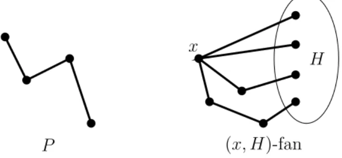
LetGbe a graph, H be a subgraph ofGand x∈V(G−H). A pathP is called an H-path if both of end-vertices of P are contained inH and all internal vertices and all edges ofP are not contained in H.

For two paths P₁ and P₂, we say that P₁ and P₂ are internally disjoint if P₁ and P₂ are edge-disjoint and all internal vertices of Pi and all vertices of P₃₋i are distinct for i= 1,2. (Possibly the end-vertex of P₁ and the one of P₂ are the same vertex.)

Let S ⊆ V(G). A subgraph F of G is called an (x, S)-fan with width l if F is a union of P₁, . . . , P_l where every P_i is a path connecting x and a vertex a_i in S with V(P_i) ∩ S = {a_i} and V(P_i) ∩ V(P_j) = {x} for 1 ≤ i <

j ≤ l. The a₁, . . . , a_l are said to be end-vertices of F. Let κ(x, S) := max{l : there exists an (x, S)-fan with width l}. For a subgraph H of G which does not contain x, we write an (x, H)-fan and κ(x, H) instead of an x, V(H)

-fan and κ x, V(H)

, respectively.

For a graph G, let p(G) be the order (the number of vertices) of a longest path in G.

(23)

x H

P (x, H)-fan

Figure 2.2: A pathP and an (x, H)-fan

2.4.2 Cycles

A cycle C is a graph withV(C) ={u₀, u₁, . . . , u_l₋₁} (l ≥3) and E(C) ={u_iu_i₊₁ : 0≤i≤l−2} ∪ {u_l₋₁u₀}. Thelength of cycle C is deﬁned asl, that is, the number of edges ofC. In particular, we call the cycle with length 3 a triangle. For a graph G, let c(G) be the length of a longest cycle in G, called thecircumference ofG.

Like the paths case, we give an orientation to C and write −→C for the oriented cycle. Forx, y ∈V(C), we denote thexy-path on−→C byx−→C y, and write the reverse sequence of x−→C y by y←C x. For− x ∈ V(C), we denote the h-th successor and the h-th predecessor ofxon−→C byx⁺^h and x⁻^h, respectively. ForX ⊆V(C), we deﬁne X⁺^h :={x⁺^h :x∈X}and X⁻^h :={x⁻^h :x∈X}. We often write x⁺, x⁻, X⁺ and X⁻ forx⁺¹, x⁻¹, X⁺¹ and X⁻¹, respectively.

a cycle C K₅ K₂,3

Figure 2.3: A cycle C, the complete graph K₅ and the complete bipartite graph K₂_,₃

2.4.3 Complete graphs and bipartite graphs

A graph G is complete if we have uv ∈ E(G) for every distinctu, v ∈ V(G). The complete graph on n vertices is denoted by K_n. A graph G is bipartite if we can partition V(G) into two partite sets V₁ and V₂ so that there are no edges joining two vertices of the same partite set. A bipartite graph G is a complete bipartite

(24)

graph if E(G) = {uv :u∈ V₁, v∈V₂}. The complete bipartite graph with|V₁|=l and|V₂|=m is denoted byK_l,m. Clearly a bipartite graphGhas no triangles. Like a bipartite graph, a graph which has no triangles is called a triangle-free graph.

2.4.4 Trees

A graph T is called a tree if it has no cycles and |E(T)| = |V(T)| −1. Let T be a tree. A leaf of T is a vertex of degree one in T. We denote by L(T) the set of leaves of T. Let r∈V(T) be a particular vertex ofT, called a root of T. Then we consider T as an oriented tree from r to leaves, denoted by −→T . We let v⁻ denote the predecessor of v along −→T . For u, v ∈ V(T), the unique path in T connecting u and v is denoted by uT v, moreover, if u ∈rT v, an oriented path u−→T v is called a path starting from u and reaching v along −→T . In particular, we also regard a path u−→T u =u consisting of one vertex u as an oriented path starting from u and reaching u along−→T .

A complete bipartite graph K₁,m is especially called astar. LetV₁,V₂ be partite sets with |V₁|= 1 and |V₂|=m. The unique vertex in V₁ is called thecenter of the star.

A graph F is called a forest if F is a graph having no cycles. A forest F which consists of a union of paths is called alinear forest. For a linear forestF, letω₁(F) be the number of components of order one in F. Moreover, if all of paths has the length 1, then F is called a matching.

a linear forest F a matching M the star K₁_,₄ Figure 2.4: A linear forestF, a matching M and the starK₁_,₄

2.5 Connectivity, toughness and blocks

A graph G isconnected if for any x, y ∈V(G), there exists a path connectingx to y; otherwise G is disconnected. Each maximal connected subgraph of Gis called a

(25)

component of G. For u, v ∈ V(G), we deﬁne a distance dist(u, v) between u and v as dist(u, v) := min

|E(P)| :P is a path in Gconnecting u and v

if u and v are contained in the same component of G; otherwise let dist(u, v) := +∞.

Let x, y ∈ V(G). We deﬁne the local connectivity κ(x, y) by the maximum number of internally disjoint paths connecting x and y. The connectivity of G, denoted by κ(G), is deﬁned by κ(G) := min{κ(x, y) : x, y ∈ V(G), x = y}. A graph G is k-connected if k ≤ κ(G). For T ⊆V(G)− {x, y}, T separates x and y if x and y belong to distinct components of G−T. Also T is called a separating set if G−T is disconnected. The following theorem is the basic one concerning the connectivity and the separating set, called Menger’s Theorem.

Theorem 2.2 (Menger [125]) Ifxy ∈E(G), then

κ(x, y) = min{|T|:T separates x and y}. In particular, if G is not a complete graph, then

κ(G) = min{|T|:T is a separating set in G}.

For the proof of Theorem 2.2, we refer the reader to [167]. By Menger’s theorem, a graph G is k-connected if and only if there exists no separating set T such that

|T|< k orG is a complete graph on at least k+ 1 vertices.

For a graph G, let ω(G) be the number of components of G. A graph G is t-tough if t·ω(G−S)≤ |S| for any S ⊂V(G) withω(G−S)≥2. Thetoughness of a graph G, denoted by τ(G), is the maximum value of t for whichG is t-tough if G is not a complete graph; If G=K_n for some n≥1, let τ(G) := +∞. In other word, ifG=Kn,

τ(G) := min

|S|

ω(G−S) :S⊂V(G) and ω(G−S)≥2

.

We say that v ∈ V(G) is a cut-vertex if G−v is disconnected. A block of G is deﬁned as a maximal subgraph which contains no cut-vertices. An end block is a block which has exactly one cut-vertex of G. We remark that each block of a connected graph is 2-connected or isomorphic to K₂.

2.6 Terminology for the speciﬁed vertices

In this section, we redefine some invariants for the specified vertices. We define the independence number, the connectivity, the minimum degree and the degree sum of the specified vertices S, as follows.

(26)

For X ⊆V(G), X is called anindependent set of S, if X ⊆S and G[X] has no edges. We deﬁne

α(S) := max{|X|:X is an independent set of S}, κ(S) := min{κ(x, y) :x, y ∈S, x=y}

and δ(S) := min{d_G(x) :x∈S}. If α(S)≥k, let

σ_k(S) := min

x∈X

d_G(x) :X is an independent set of S with |X|=k

; otherwise σ_k(S) := +∞. For r≥k, if α(G)≥r, let

σ_k^r(S) := min{Δ_k(X) :X is an independent set of S with |X|=r};

otherwise σ_k^r(S) := +∞. The following proposition is the same one as Proposition 2.1 ifS =V(G).

Proposition 2.3 (i) If k ≤ l, then _k^lσ_k(S) ≤ σ_l(S). In particular, lδ(S) ≤ σ_l(S).

(ii) If k ≤l≤r, then^k_lσ_l(S) ≤σ_k^r(S). In particular, σ_k(S)≤σ_k^r(S).

It follows from Theorem 2.2 that the similar result for a fan holds.

Lemma 2.4 Let G be a graph and let S ⊆ V(G). Then for any x ∈ S, there exists an x, S− {x}

-fan with width at least min

|S| −1, κ(S)

. In particular, κ x, S− {x}

≥min

|S| −1, κ(S) .

(27)

Chapter 3 Hamilton cycles and cyclability

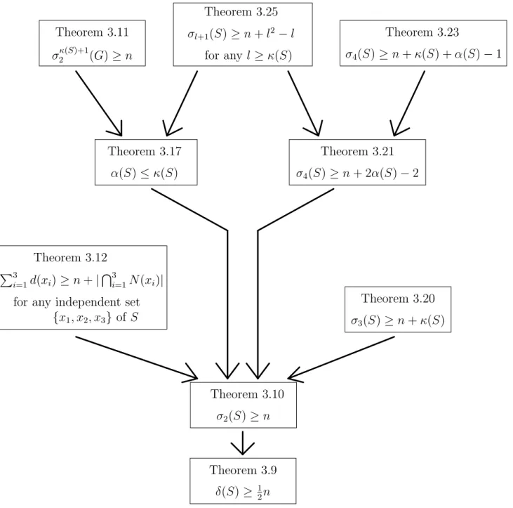
A hamilton cycle problem, determining whether a given graph has a hamilton cycle or not, is one of the most important problem in Graph Theory, because of the relationship to some other problems or topics. In this chapter, we introduce some sufficient conditions for the existence of a hamilton cycle. In particular, we concentrate on degree conditions or independence number conditions. In addition to a hamilton cycle problem, we consider a cyclability problem, determining whether a given graph has a cycle passing through given vertices or not. In Sections 3.1 and 3.2, we show some results on hamilton cycles and cyclability, respectively, and in Section 3.3, we show the relationship between these results. In Section 3.4, we prove Theorem 3.23, which is a new sufficient condition for specified vertices to be cyclable.

The contents of this chapter are based on the paper [135] “A degree sum condition concerning the connectivity and the independence number of a graph,” joint- work with T. Yamashita.

3.1 Results of Hamilton cycles

A cycle C in a graph G is called ahamilton cycle ifV(C) = V(G). In particular, a graph which has a hamilton cycle is called hamiltonian. The following theorem is the most classical one giving a suﬃcient condition for a graph to have a hamilton cycle.

Theorem 3.1 (Dirac [41]) LetG be a graph of order n≥3. Ifδ(G) ≥ ¹₂n, then G has a hamilton cycle.

Ore considered the following result with a σ₂(G) condition. By Proposition 2.1 (i), this is a generalization of Theorem 3.1.