Robust H∞/ μ Control and Uncertainty Description of Mechatronic Systems
著者 滑川 徹
year 1997‑03‑25
URL http://hdl.handle.net/2297/30579
,
( l 〉
博 士 論 文
メカ卜口ニクスシステムの不確かさの記述と 口バスト
H ∞
/μ制御に関する研究金沢大学大学院自然科学研究科
滑 川 徹
Contents
s
N
x
Acknowledgment 1 Introduction
1.1 Background . . . .
1.1.1 Control of Real Physical System . . . . 1.1.2 Uncertainty and Robustness . . . .
1.1.3 Previous Work ...
1.2 Goal and contribution of this paper . . . . 1.3 Organization of the thesis . . . .
2 Robust Control and Uncertainty Description
2.1 Framework of the Robust Control . . . . 2.1.1 Modeling and U ncertainty . . . . 2.1.2 Uncertainty Descriptions . . . .
2.2 ff.. Control Theory . . . .2.2.1 Problem Formulation . . . . , . . . . 2.2,2 Characterizing all solutions . . . .
2.3 pa-Analysis and Synthesis . . . .2.3.1 Structured Singular Value pa . . . . 2.3.2 Linear Fractional Transformations...
2.3.3 Well posedness and Performance for LFT's 2.3.4 Robust Stability. . . .
2.3.5 Robust Performance . . . . 2.4 Quantity of Uncertainty . . . . 2.4.1 Iterative Design . . . . 2.4.2 How to make a set G . . . .
v
1 1 2 3 3 4 5
8
8 8 10 13 l3 15 19 19
22 23 24 25 27 27
28i
ii
3
4
Robust Control of Magnetic Suspension Systems
3.1 pa-Synthesis of an Electromagnetic Suspension System . . .
3.1.1 Introduction . . . .3.1.2 Experimental Setup . . . .
3.1.3 Model of EIectromagnetic Suspension System ...
3.1.4 Design . . . .
3.1.5 Experimental Results . . . . 3.1.6 Conclusions . . . .
3.2 Gain Scheduled Hoo Robust Control of a Magnetic Bearing 3.2.1
3.2.2 3.2.3 3.2.4 3.2.5 3.2.6 3.2.7
Robust
4.1 4.2
4.2.1 4.2.2
4.3 Model
4.3.1 4.3.2 4.3.3
4.4
4.4.1 4.4.2 4.4.3
4.54.5.1 4.5.2 4.5.3
Control of Active Pantograph
Introduction Experimental Eq
Control System Design
Experimental Results
Introduction...
Modeling ...
H.. G ain Scheduling . . . . Controller Design . . . . Simulation Results . . . . Experimental Results . . . .
Conclusion...
Systems
ulpment...
Pantograph Experimental Equipment ...
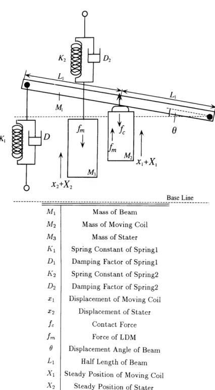
Digital Control System . . . . ing .
Differential Equation of Beam, Mover and Stater
state-space model . . . .Parametric Uncertainty and Neglected Dynamics
Review of pt-synthesis . . . . Construction of the Gen er alized P lant . . . . . Controller Design . . . .
H.. controller based on differential game theory
Experiments...
Consideration . . . .
•
CONTENTS
32 32 33 33 35 42 47 49 50 50
5155 59 64 67 68 72 73 74 74 75 76 76 79
8184 84 85 88 89 89 90
91CONTENTS
5
4.6 Conclusion...
Robust Control of Robot Manipulators
5.1 pa-Synthesis of the Robot Manipulator Using Exact Linearization . .
5.1.1 Introduction . . . .5.1.2 Robot Manipulator Dynamics and Uncertainty Modeling . . 5.1.3 Control System Synthesis . . . .
5.1.4 Application of pa-synthesis for a Robot Using DSP ...
5.1.5 Experimental Results . . . .
5.1.6 Conclusion . . . .5.2 Robust H. Control of Robot Manipulators considering structured
tamtles...
5.2.1 5.2.2 5.2.3 5.2.4 5.2.5 5.2.6 5.2.7
5.3 pa-Synthesis of Robot Manipulators U sentatlon
5.3.1 5.3.2 5.3.3 5.3.4 5.3.5
5.4 Consideration 6 Conclusions Bibliography
uncer-
Introduction...
Robot Control System ...
Robot Dynamics ...
ActuatorDynamics...
Design ...•••••••••••••••••••••
Experiments...•.•••
Conclusions...•....
sing Linear Parameter Varying Repre-
Introduction...
Robot Dynamics ...•.•.•
Control System Design . . . .
Simulation Results ...
Conclusion...••••••••••
' and Investigation for Approaches . . . .
iii
95
96
96 97 98 100 102 106 108
112 112 113 113 115 120 123 125
128 128 129 133 135 136 137
138
143
Acknowledgment
First and the most, I would like to begin by thanking my advisor Professor Fumio Matsumura. His guidance and excellent supervision during my doctoral work has been
invaluable.I would also like to thank my advisor Professor Masayuki Fujita for his fruitful dis- cussions and valuable suggestions. His excellent advice on my thesis topic were the most
helpful.I would like to thank the members of my thesis committee, Professor Naofumi Fujiwara, Professor Yoshitsugu Kamiya, and Professor Kazuo Tanaka for their valuable suggestions and recommendations on my thesis.
I would also like to thank all the members of Matsumura's and Fujita's laboratories for providing an enjoyable and stimulating work environment, especia}ly to Mr. Kubo and Mr. Hatake, with whom I had a plenty of exciting discussions.
My special thanks go to my family and friends for their support through my many years here at Kanazawa University and JAIST. This path would have been much more difliicult
had it not been for you all.Again, it is my pleasure to thank all these people for the precious and invaluable experiences I gained during this doctoral work in Kanazawa.
Kanazawa Toru Namerikawa October, 1996
v
Chapter 1
Introduction
1.1 Background
The field of control engineering has developed over this century from its origins in the investigation of feedback amplifiers, into a broad discipline concerning various issues of modeling, dynamics, optimization and feedback control. On one side lie complex engi- neering problems, such as regulation in chemical processes, trajectory tracking for robot manipulators, stabilization of high performance aircraft and magnetic suspension systems, or dynamics of queueing systems. On the other side lie tools from virtually every mathe-
matical discipline, from dynamical systems and differential geometry to stochastic processes and operator theory. In the middle of this, the task of the control theorist is to abstracta problem of significance in engineering, cast it in an appropriate mathematical setting, and derive a solution, by which is meant a practically computable method of evaiuation of the problem at hand. This eclectic mix of disciplines has made control theory the home of people who have found it diMcult to choose between the fascinating worlds of engineering and mathematics.
While engineers are mainly concerned with real-world problems, and mathematicians with the logical consistency of their abstractions, it is the job of those who attempt to
apply mathemat,ics to the real world to deal with the fundamental gaps between theory and practice, which reflect themselves in uncertainty about the behavior of a real system when one is given a mathematical prediction. This is particularly the case for control theory, which treats the question of feedback, a technique used by both natural and artificial
systems to obtain reliability in spite of faulty predictions. A property of design feedbackcompensator will effectively reduce the sensitivity of the systems to certain sources of
1
'2
CHAPTE]R1. INTR.ODUCTION
uncertainty, but at t,he expense of increased sensitivity to order unniodeled effects, e.g., in an()ther frequency band. Coiise,que'ntly. a, t/heory of feedback rnust l)rovide nieans to quantify these tradeoffs, vvrhich can onl.v be a,chieved if in addition to a niatheniatical inodel, one utilizes sonie forn) of quantification of n'iodel uncertainty.
[I"his thesis is concerned with the robust Iil..,/LL control of real niechatronic systeins from the point of view of the effect of uncertainty. The fundamental challenge in this area ha,s been tio refine as much a,s possible the uncertainty deg.cription in a rnodel of a coniplex system, compatible with t,he possibility ()f a tractal.)le evaluation of it,s effect,. I describe a set of inodels and perforin Lvorst-case analysis b.y using ff.,/tt, synthesis and analvvsis, a. i}d evaluat/e its effe('ts by inechatronic experiinents.
1.1.1 ControlofRealPhysicalSystem
No inatheinatica} systen) can exactly inodel a, real physica,1 systeni. For this reasoii w•e niust be aware of how rnodeling errors niight a,dve.rsely affect the stability and perforniance
of a control system. In the physical sciences, very accurate niodels in themselves are the
objective. To obtain these physical laws, one often distills the phenomenon to its siniiplest forin. In this c()ntext. uncertainty is interpreted in a, narrow sense as referring to t/he liinits in the predictive powcr of the best availa,ble models.I odels play a different role in engineering science; they are tools employed in analysis, simulation and design of complex, artificial systems. Consequently, rriodels fidelity must be traded off with the complexity of the modeling process and the tractability of the resulting
mathematical and computationa,1 problems. From this point of view the best model is the
siinple,st sun)niary o{" t,lie rnain aspects of the physical systern which are relevant to the eiigiiieei'iiig (luestioii at haiid.'The issue of uncertainty is at the main theme of cont,rol engineering, since a feedback configuration can significantly affect the sensit,ivity of t,he sy, stein behavior to unce.rta,inty at the coniponent Ievel. This is the nia,in n]otivation for the construction ()f feedl)a(:k f .vstenis,
but also the main potential danger as unmodeled effects can. Consequently, to perform
good designs, the control engineer must• be furnished v"'ith rich descriptions of uncertainty and tools to a,ssess their impact in a complex system.It is very iinport,ant a,nd difficult• to t/reat various niodels of plant uncertainty. H.,/tt, control has a good structure t,o treat/ uncertainty. In this paper robust stability, stabilit,y in the face of p}ant uncertaint.y, in stuclie.d using the srriall-gain theorem and Nyquist stability
CHAPTER 1. INTRODUCTION
3criterion. Further robust performance,
is also discussed.guaranteed tracking in the face of plant uncertainty
1.1.2 Uncertainty and Robustness
A fundamental problem in t,he design of control systems is to cont,rol accurately the out- puts of a system(plant) whose dynamics contain significant uncertainties. For example,
characteristic of niagnetic force is so complex that analysis of this force is very difficult andno mathematical models can express the exact behavior of it. In the latest few decd"des
there have been great advances in the. theory for the design of robustly uncerta,inty-tolerant feedback control systerns [9]. rl"he probleni in robust feedba,ck control systein design is t,o synthesize a control Iaw whicb maintains system st,ability and perf()rma,nce and error signals to within pre-specified tolerances despite the effects of uncertaint,y of the systeni [11].Uncertainty may take a lot of forms but among the most/ significant are
e Paramet,ric Uncertainty e Disturbance Signals
o Unmodeled Linear Dynamics e Unmodeled Nonlinear Dvnamics v
Uncertainty in any form is no doubt the major issue in most control system designs
This mot,ivates researchers to seek a quantit/at,ive measure for the size of the uncertaintye.g., the U2 and H,., norm, the real/complex structured singular value LL, and so on.
'
1.1.3 Previous Work
It is a few decades since Hoo/LL control theory has been studied extremely as a design tool [6] for the robust controlled systeni. H../LL control theory provides a direct, a,nd reliable procedure for synthesizing controller which optiinally satisfies t,he U.. norn)/ structured singula,r va,lue IL specifications. This method has an advantage to quantify the effects of
unmodeled dynamics and to clarify the stability margin.
rl"here are so many theoretical results and papers in robust control fields. Nowadays
the most challenging issue is its app}ication to real physical systems. Applications of H..control to industry is now expect/ed.
4
CHAPTER1. INTRODUCTION
Many application papers have been published, but almost of them employ poor control problems and groundless generalized plants. Just a few papers focus on real uncertain-
ties/perturbations.Doyle and Balas applied H../pa control theory to a flexible structure[5], and they in- troduced the large-scaled and complicated interconnection structures for the plant. Hyde and Glover also controlled a VSTOL by using H. control law [29][30][31]. Steinbuch used
pa-synthesis for control of a compact disc player [75].In order to design a H../pa conirol system, it is very important to choose suitable design
parameters for ea,ch control problem and a plant. The problem is how to construct the generalized plant• and how to select design paramet/ers. In the previous research, even as the above papers, tuning of the design parameters depended on experimental/simulated trial and error. Tuning of design parameters, especially frequency weighing functions is very heavy burden for control design engineers. Development of systematic tuning method
of design parameter is now ex. pected.Further, in the previous works, physical limit of allowable perturbation for robust sta- bility/performance was not clear. NVeightings for uncertainties werejust design parameters,
but ph.vsical stability and performance margins against perturbations were not considered.
The second problem is that there are just a few application papers of U./pa control theory in real nonlinear mechatronic systems, as robot manipulators. Robot dynamics is highly interfered, nonlinear, and complicated. Experimental evaluation is now expected.
Hashimoto and Asai treated H. control or pa syrithesis of a robot manipulator, but dynamic couplings between joints were not considered, and the uncertainties caused by modeling
errors was treated the external disturbance[27][4].1.2 Goal and contribution ofthis paper
The goal/contributions of this paper is as following three items.
e As described in the last subsection, in order to design a H../pa control system with better properties, it is very important to choose design parameters suitably, and we expect them to be selected more systematically and meaningfully.
The first goal of this thesis is a proposal of a more systematic quantification of the
model uncertainty.
CHAPTER 1 . INTRODUCTIOIV'
5We make a set of plant model and quantify the rnodel uncertainties, and clarify the
limit of allowable class of perturbation for robust stability and performance.e There are just a few papers of Hoo/pt application in real robot manipulator con- trol field, because robot dynamics is hjghly i'nterfered, nonlinear, and complicated.
Experimental evaluation is now extremely expected.
The second goal of this thesis is a robust control of robot manipulators by using H..
control theory.
We guarantee the robust stability of the robot manipulator control system against model perturbations and dynamic couplings.
Further we apply the robust Hoo/pa control theory to a robot manipulator in order
to evaluat•e its effectiveness for nonlinear systems.Our approaches taken here are as follows.
- pt-synthesis with exact linearization
- constant scaled H.. control considering structured uncertainties - pa-synthesis using linear parameter varying representation
e Third, we apply the advanced H../pa control theory to real mechanical systems, then evaluate the performance of the control theme and expressive ability of LFT against
various forms of uncertainties.We experimentally show that H../LL control theory has a very good framework to
treat uncert,ainties, in order to guarantee robust stability and robust performance.Our mechatronic plants employed to evaluat/e robust control theory are as follows.
- magnetic bearing: linear, MIMO, unstable
- pantograph system with linear DC motor: linear, SISO, stable, but highly oscillatory
- robot manipulator: nonlinear, MIMO, stable
1.3 Organizationofthethesis
Organization of the thesis is represented in the diagram of Fig.1.1 This thesis has a small hierarchy.
6
CHAPTER 1. INTRODUCTION
1) Framework of the Robust Control 2) Hoo Control Theory
3) " -Analysis and Synthesis 4) Quantity of Uncertainty
1) " -Synthesis of EMSS
,
2) Gain Scheduled Hoo Control of MB
Chapter 3
Chapter 2
Robust Control of
APS
Chapter 4
Linear Systems
Figure 1
1 l I I 1 t 1 I l 1 1 l l 1 l I
1) pt -Synthesis of RM Using Exact Linearization 2) Robust Hco Control of RM 3) u -Synthesis of RM Using LPV Representation
.1: Organization of the thesis
Chapter 5
Robot Manipulator (Nonlinear Systems)
Chapter 2 explains a general robust control problem and asserts a main approach to quantify uncertainties. In this chapter, at first, framework of the robust control is de- scribed, especially about modeling, uncertainty, and uncertainty descriptions. Then H.
control problem/theory, and pa-analysis and synthesis approach is introduced. Mathemati-
cal definitions and theorems are also given in Chapter 2. The article entitled "Quantity of uncertainty" is written in section 2.4, which is a main assertion and concept of this thesis.Then we apply this methodology proposed in section 2.4 to three mechatronic systems,
and results are presented in chapter 3, 4, and 5, respectively.In chapter 3, robust control of magnetic suspension systems is described. Section 3.1 is
entitled with "pa-Synthesis of an Electromagnetic Suspension System". And section 3.2 is entitled with "Application of Gain Scheduled H.. Robust Controllers to a Magnetic Bearing
". In section 3.1, we show a result of pa-synthesis approach with a simple SISO magnetic suspension system. Section 3.2 is an extension version of section 3.1. Here the controlled plant is a MIMO(four inputs, four outputs) multivariable magnetic bearing system. We derive an advanced gain scheduled H. control method by utilizing free parameter of the controller, and applied the method to this magnetic bearing system.
In chapter 4, robust control of active pantograph system by using linear DC motor, is
CHAPTER 1 . INTRODUCTION
7described. Here we considered both parametric uncertainties and dynamical uncertainty which is an unmodeled uncertainty of the piant in the modeling process, and construct the interconnection structure by LFT. For controller design, we employ thsynthesis approach.
The experimental results show the effectiveness of the proposed modeling and design by a comparison with a conventional modeling and H. method.
In Chapter 5, robust H.. control of robot manipulators is discussed. This chapter is constructed with three main sections, and the following approaches are taken in this
chapter.e pa-synthesis with exact linearization
e constant scaled H.. control
e linear parameter varying representation approach
Robot manipulator dynamics is written with nonlinear ordinary differential equation.
This makes robot manipulator control complicated.
In the first approach, we employ the exact linearization, and then for the obtained
linearized plant, we apply the linear pa-synthesis method. In the second approach, we dividethe original nonlinear dynamics with linear nominal model and nonlinear perturbation.
Then we used constant H.. problem and small gain theory to guarantee the robust stability for nonlinear perturbation. The third approach utilize the recent advanced topics, gain scheduling for linear parameter varying system. Dynamics of robot manipulator with flexible links is written as linear parameter varying system. We derive the LPV equation
of the plant and pa-synthesis approach is used for control system design.In chapter 3 and 4, we treat linear systems and in chapter 5 our plant is a robot ma- nipulator, which is a typical nonlinear system. From section 3.1 to 3.2, complexity of the plant is extended from SISO to MIMO. From section 3.1 to chapter 4, description of the model uncertainty is extended from the unstructured one to the structured.
Finally, we conclude this thesis in Chapter 6.
Chapter 2
Robust Control and Uncertainty Description
Recently H.. and pt-synthesis theories have been developed [12] [13]. The H.. theory
provides a direct, reliable procedure for synthesizing controller which optimally satisfiessingular va,lue loop shaping specifications. Robust stability in the H.. control framework
is guaranteed by the small gain theorem, this theorem provides reliable results for unstruc- tured uncertainties, but it is well knovv'n that it gixres conservative evaluations for structureduncertainties as robust performance problems.
To improve this property, by using the multivariable Nyquist stability criterion, the pa-analysis and synthesis method provides a, less conservative valuation for a structured uncertamty.
2.1 Framework of the Robust Control
2.1.1 Modeling and Uncertainty
Any mat•hematica,I models can not exactly express a behavior of the real physical system.
For this reason we must be aware of hovv' modeling errors might adversely affect the stability
and performance of a control system.
Fig. 2.1 shows a,n usual framework of the control system design and real-time control.
Generally we derive a model for the real plant and by using the obtained model, a con- troller is designed. We implement this controller and apply it to the original real plant.
But the contro}ler was just optimized for the 'model' and not for the real system. The
8
CHAPTER 2. ROBUST CONTROL AIVD UNCERTAINTYDESCRIPTION
9uncertainty between the real physical system and the nominal model depresses the stability and performance of the closed-loop system.
In the physical sciences, very accurate models are the objective in themselves. To obtain these physical laws, one often distills the phenomenon to its simplest form. In this context, uncertainty is interpreted in a narrow sense as referring to the limits in the predictive power
of the best available models. For example, the uncertainty associated with prediction in a chaotic systems, or the uncertainty principle in quantum mechanics refer to fundamental
limitations in predictability.Models play a different role in engineering science; they are tools employed in analysis,
simulation and design of complex, artificial systems. Consequently, models fidelity must be traded off with the complexity of the modeling process and the tractability of the resulting mathematical and computational problems. From this point of view the best model is the simplest summary of the main aspects of the physical system which are relevant to the engineering question at hand, Correspondingly, the term "uncertainty"
is used here in a broader sense: is not only describes what one is fundamentally unable to predict, but also, and often predominantly, many aspects of the system which one has chosen to neglect or simplify. For uncertainty in this broad sense, there is by definition no detailed model, but often the modeling process yields a crude description which allows one to assess its implications on the overall system. There descriptions of uncertainty appear commonly and in various forms in engineering models, whatever they result from
"black box" system identification techniques, from "first principles" models obtained by
application and simplification of physical laws, or a combination thereof.As remarked in Introduction, the issue of uncertainty is at the heart of control engi-
neering, since a feedback configuration can significantly affect the sensitivity of the systembehavior to uncertainty at the component level. This is the main motivation for the con- struction of feedback systems, but also the main potential danger as unmodeled effects can, for example, lead to instability. Consequently, to perform good designs, the control engineer must be fumished with rich descriptions of uncertainty and tools to assess their impact in a complex system. It should be clear from the nature of these descriptions that
no hard "guarantees" can result from this assessment; ultimately, the control engineer mustbe the final mediator between the mathematics and the real system.
In Fig. 2.1, the uncertainty A causes various problems when we design a controller and
control of a real physical system. We know A is a gap between the real physical system
and the model, but we have to discuss the A in detail. Our problems are as follows.
10
CHAPTER 2.
'NNN)th,
ROBUST CONTROL AND
1-"eA jer--
UN CERTA INT Y DES CRIP TION
W A
zReal Physical
System N N- .
7
,,,,,,ef'
1
Modeling
Identification u
Nominal Model
y
Real-Time Control
Design
Controller
Figure 2.1: General framework of design and real-time control e What is physically included in A ?
e How is A expressed?
e How can we measure/quantify A?
These problems are discussed in the following sessions.
2.1.2 UncertaintyDescriptions
Traditional methods for uncertainty characterization in dynamical systems include para- metric uncertainty, disturbance signals, and system perturbations to account for unmodeled dynamics. We now describe how these typically arise in modeling. For more motivation
we refer to [14].
Parametric Uncertainty
Parameters are present in most engineering models, representing a rea} physical quantity which can be assumed to be a real constant within the range of validity of the model. The following are some reasons for uncertainty in the value of a parameter.
o It could be obtained indirectly from experimental data, which leads to statistical deviations.
cHAPTER 2. ROBUST CONTROL AND UNCERTAINTYDESCRIPTION 11
e It could represent a standardized component (e.g., electrical resistor) subject to man-
ufacturing tolerances.
e It could represent an operation condition which varies in an unforeseen way. A constant parameter is a reasonable model when this variation is very slow (e.g., ambient temperature). In other cases the rate of variation of the operation condition is comparable to the modeled dynamics (e.g., aerodynamic eMcient of an airplane executing a sharp maneuver). In this case a time-varying parameter may be preferred.
The most straightforward representation of parametric uncertainty is in terms of an
interval of the real line, such asp == po + k,6, 6 E [-1, 1].
In models of linear dynamical systems, it is common to encounter rational dependence of a transfer function on an uncertain parameter.
Disturbance Signals
Another commonly used method to account for model uncertainty is the injection of dis- turbances, which are thought of as generated by an external process. Some ways in which
they arise aree To account for microscopic fluctuations which are not included in a large scale model(e.g., wind turbulence, thermal noise in a circuit).
e To describe more systematic effects which are neglected in a simplified model (e.g., ripple in a voltage source, quantization error in an A/D converter).
e In identified models, frequently used as an error signal needed to account for the data.
The two standard choices for characterization of disturbances are in terms of a stochastic process, or in terms of a set of signals.
Unmodeled Linear Dynamics
The most commonly used dynamical system model for purposes of control is linear, finite
dimensional time invariant system, which is equivalent to a set of linear ODEs, preferably ofi2 CHAPTER 2. ROBUST CONTROL AAJD UNCERTAINTYDESCRIPTIO.ZV
low order. Assuming for now that nonlinear effects are negligible, a low order approximation amounts to neglecting linear dynamics, in particular distributed effects.
This uncertainty is expressed as follows e Additive Uncertainty:
H=P+ W,AW,.
e Multiplicative Uncertainty:
H = (I + W,AW,)P.
e Coprime Factor Uncertainty:
H = (?VI + AM)-i(N + A.).
Unmodeled Nonlinear Dynamics
If nonlinear are very significant in the range of operation, the model itself must be chosen to be nonlinear. Uncertainty descriptions for nonlinear models are not very well developed, and are one of the main open challenges for a satisfactory theory of robust nonlinear control.
CHAPTER 2. ROBUST CONTROL AND UNCERTAINTYDESCRIPTION 13
2.2 H. ControlTheory
Robust stability against unstructured uncertainty in H.. control framework is guaranteed
by small gain theorern. Detailed definition and proof are written in [87].In this section, the results by Keith Glover and John C. Doyle[25] is introduced.
There are so many other state-space formulae for all stabilizing controllers that sat- isfy an H.. norm bound, but this one is the original and the most famous and typical characterization, which is emp}oyed by MATLAB and MATRIXx.
2.2.1 ProblemFormulation
The most general block diagram of a control system is shown in Figure 2.2 . Where P is
the generalized plant and Is' is the controlier.Since the work of Zames[86], there has been much interest in the design of feedback
controllers for linear systems that minimize the H.. norm of a specified closed-loop transferfunction. Let a linear system P(s) be described by the state equation
th (t)=Ax (t)+Biw(t)+B2u (t), (2.1)
z(t)= Cix (t) +Diiw (t)+Di2u (t), (2.2)
y(t)= C2x (t)+D2iw (t)+D22iL (t). (2.3)
where
x(t) E R", w(t) E RMi, iL(t) E RM2, z(t) E RPi, y(t) E RP2
The generalized plant P contains what is usually called the plant in a control system plus all any frequency-dependent weighting functions.
The signals, w(t), z(t), y(t), and zL(t) are vector-valued functions of time. x(t) is the
state vector. The components of
w : are all the exogenous input: reference, disturbances, sensor noises, and so on.
z: are all the signals we wish to control: tracking errors between reference signals and
plant output, actuator signals whose values must be kept between certain limits, and
so on.
14
y u
:
:
CHAPTEJR2. R.OBUSTCONTROLAND
w
---)))-
P u
UN CERTA INTY DES CR IP TIOIV
Z
K
y
Figure 2.2: Most general Control System
contains the outputs of all sensors.
contains all controlled inputs to the generalized plant.
The transfer functions will be denoted as follows
p(,) ,= (pP,il pPli)
- (S,'l S;;)+[g,'i2](si-A)-i[B,
s
A
Ci C2
Bi B2
Dll D12 D12 D22
sc
The diagram is also referred to as a linear fractional transformation(LFT
2.3.2) on A' and P is called the coefficient matrix for the LFT.
transfer function from w to z is denoted by T..
.11 li(P, K) := P,, + P,,K(I - -P,,K)
The H.. control problem is then to choose a controller K(s) system internally stable ( see [25]) and minimize
(2.4)
B,] (2.5)
(2.6)
(2.7) ; see subsection The resulting closed-loop
== .7'li(P, K), where
-i P,,. (2.8)
, that makes the closed-loop
Il'11Ti(P,K)11oo,
cHAPTER 2 ROBUST CONTROL AIVD UNCERTAINTY DESCRIPTION 15
where
11Gll.. = supa(G(]'w)) (o := maximum singular value). (2.g) w
We will in fact be considering the closely-related problem of finding all stabilizing K such that
ll.JEIi(P, K)ll.. s{l7 (2.Io)
for some prespecified 7 E R
It is the purpose of the present note to give a state-space parametrization of all con-
trollers that satisfy (2.10); this solution will only involve two algebraic game-type Riccati equations, each of degree n[25] [12].2.2.2 Characterizing all solutions
This section will give a state-space characterization of all stabilizing controllers K(s) such
that ll.1Ti(P,K)".. < 7. We will make the following assumptions that are also typically made in the corresponding LQG problems.
Assumption 2.1
e (Al) (A,B2)is stabilizable e (A2) (C2,A) is detectable.
e (A3) rank Di2 = m2 (Di2 is full column rank.) e (A4) rank D2i =p2 (D2i is full row rank.)
e(As) rank [A-c('WI DBi22]=n+m2 Vw
( full column rank) o
Pi2 does not have any zeros on the imaginary axis.
o
There are no unobservable poles of (A - B2Di2Ci, DiÅ}2Ci) on the imaginary axis•
e (A6) rank [A -c12'tuI DB2',]=n+p2 Vw (full row rank) o
P2i does not have any zeros on the imaginary axis.
o
There are no uncontrollable poles of (A - BiD2tiC2, BiD2ii) on the imaginary axis•
16 CHAPTER 2. ROBUST CONTROL AND UNCERTAINTYDESCRIPTION
e (A7) A scaling of u and y, together with a unitary transformation of w and z, enables us to assume without loss of generality,
Di2 == [I9,], D2i == [o I,,], D22 ==o
Assumptions (Al) and (A2) are required for the existence of a stabilizing K. These
assumptions are equivalent that the real plant is stabilizable and detectable, and the weight- ing functions are stable.(A3) and (A4) are sufficient to ensure that the controllers are proper, but there are sen-
sible problems when it is violated. Di2 = Pi2(oo), D2i = P2i(oo), then these assumptions mean Pi2 and P2i do not have any zeros at 7' = oo. If these would be deleted, expansion of equations are more complicated.
(A5) and (A6) are need for spectral factorizations.
(A7) ensure that the solution to the corresponding LQG problem is closed-loop asymp-
totically stable, and is also convenient for the present problem.The main result is now stated as follows.
Theorem 2.1
For the system described by (2.1)-(2.3) and satisfying the assumptions (Al)-(A7), There
exists an internally stabilizing controller Isr (s) such that l1.1 li(P, K)1I.. < or if and only if(i) 7 > max(0[Diin, Dni2],0[Dliii, Di*i2i]), where
D,,-[Sli,ll D.llli],
Dml E R(Pi-M2)Å~(Mi-P2),Dll12 E R(Pi'M2)XP2,Dl121 E RM2Å~(Mi-P2), Dl122 E RM2XP2.
and
(ii) there exist X.. ) O and Y.. 2 0 satisfying (2.11) and (2.12) respectively and such that
Amax ( Xoo Yoo ) < ry 2,
where
XOO == RiC ([- c4* c, -0A*] - [- cE. D,.] R-'i[D le Ci B' ])' (2'11)
Yoo = RiC([".,i;,'Br -OA]-[-B9b;,]R-'[DeiBr C]), (2.12)
cHAIJ)T.ER 2. .R,OBUST COIVTROL Apt'D UAJ/(.E]RTAI,IVTYDII]SCRU)TION 17
R= Dr.Di.'P2(I/Mi :], Die=[Dii Di2] (2'13) R ., D.,D:,-[AX2oiPi g], D.,=[Sll] (2.i4)
The solution X.. and Y.. to an algebraic Riccuti equation (ARE) are denoted via its Hamiltonian matrix as (2.11) and (2.12).
Theorem 2.2
Given that the conditions of Theorem 2.1 are satisfied, then all rational internally stabi- lizing controllers A' (s) satisfying llJZ ;i(P, A')1Ioo < 7 are given by
1'-s,' := .7 li(I"s',".,<l>) = IT•s,'ii + I-s,ii2Åë(I- .l-is,f22<I>)-i1'"s,'2i, (2.15)
Åë E R-Hoo, s•t• llÅëlloo < ty, where
is'. :- klll ;llli]2 • (2•i6)
A= A+ HC+B,b,-,i O,, (2.17) B, = -H,+B,b,-,iD,,, (2.ls)
B, = (B,+H,,)b,,, (2.lg) O, = F,Z+b,,b,-,iO,, (2.2o) 02 = -b2i(C,+F,,)Z, (2.21)
Dii = -Dii2iDIm(72I-DmiDrm)-iDm2mDii22, (2•22)
bi2 E RM2XM2 and b2i E RP2XP2 are any matrices (e.g., Cholesky factors) satisfying
bi2bi'2 == I'Dn2i(72I-DliiiDim)-'D:i2i, (2•23) b2'ib2i = J-Dli2i("x'2I-DimD;m)-'Dn2i, (2.24)
Fl1
F : Fi2 =-R-'[Dr.Ci+B'Xoo], (2.25)
F2
H = [Hii H,2 H,]=-[B,D:,+Y.C*]R-i, (2.26)
Z == (I-7ny2YooXoo)-', (2•27)
A B,B,
D,,b,,
b,,o
18 CHAPTER 2. ROBUST CONTROL AND UNCERTAINTYDESCRIPTION
FII E R(Mi'P2)Xn, F12 E RP2Xn, F2 E RM2Xn, Hn E RnX(Pi'M2, H12 E RnXM2, H2 E RnXP2.
F and H are called the 'state feedback' and 'output injection' matrices, respectively. In (2.16), Åë(s) is called free parameter. And if Åë(s) == 0, then controller K(s) should be
Kii(s) from (2.16). Kii(s) is generally called 'central controller'. The central controller isformulated as
Is'11(s) ==
A B,
Oi b,,
(2.28)cHAPTER 2. ROBUST COAITROL AND UNCERTAINTYDESCRIPTION 19 2.3 pa-Analysis and Synthesis
The small gain theorem provides reliable results for unstructured uncertainties, but it is
well known that it gives conservative evaluations for structured uncertainties as robust per-formance problems. To improve this property, by using the multivariable Nyquist stability criterion[41], the pa-analysis and synthesis method provides a less conservative valuation
for a structured uncertainty.2.3.1 Structured Singular Value pa
In this section I devote to defining the structured singular value, a matrix function denoted by pa [13]. Consider matrices M E C"Å~". In the definition of pt(M), there is an underlying
structure A, (a prescribed set of block diagonal matrices) on which everything in the
sequel depends. For each problem, this structure is in general different; it depends on theuncertainty and performance objectives of the problem. Defining the structure involves specifying three things; the type of each block, the total number of blocks, and their dimensions.
There are two types of blocks-repeated scalar and full blocks. Two nonnegative in- tegers, S and F, represent the number of repeated scalar blocks and the number of full
blocks, respectively. To bookkeep their dimensions, we introduce positive integers ri,...,rs;mi,...,mF. The i'th repeated scalar block is ri Å~ ri, while the ]"th full block is mj Å~ mj.
With those integers given, we define A c CnX" as
A == {diag[6il.,,•••,6sl..,Ai,...,AF] : 6i E C, Aj E CMJXM)} (2.29) For consistency among all dimensions, we must have
SF
2ri +2mj =n (2.3o)
i=1 j'--1
We will often need norm bounded subsets of A, and we introduce the following notation
BA={AEA:0(A) -<d. 1} (2.31)
Note that in (2.29) all of the repeated scalar blocks appear first. This is just to keep the notation as simple as possible, in fact they can come in any order. Also, the full blocks do not have to be square, but restricting them as such saves a great deal in terms of notation.
2o CHAPTER 2. ROBUST CONTROL AfX"rD UIS"ÅéERTAINrTYDESCRIPTION
Definition 2.1 [13]
For iV E CnX", xLA(A,I) is defined
1
pa"(M) := min{o (A) :AE A, det (I- MA) = o} (2'32)
unless no 2x E A makes I - MA singular, in which case paA (M) :== O.
An alternat,ive expression for /LA (Al) follovv's froni the definition(2.32')).
paA(M) := .Il}gx.p(MA) (2.33)
From (2.33) continuity of the function LL: C"Å~" - R is apparent. In general, though,
the function LL: C"Xn -> R is not a norm, since it doesn't satisfy the triangle inequality.However, for any a E C, xL (aAI) = lalpa (A'1). so in soine sense, it is related to how "big"
t;he matrix is in a norm sense.
We can relat,e LL (ct.M) to familiar linear algebra quantities when A is one of two extreme
set,s.
e IfA= {6I :6G C} (S z 1, I7 = O, ri = n), then pt(.M) =p(A4), the spectral radius of M.
e If A= C"Å~" (S = O, F == 1, mi = n), then pt (M) =0(M).
For a general A as in (2.29) we must have
{6I. :6E C} cAc C"Xn (2.34)
Hence directly from the definition of pa, and the two special cases above, we conclude
that,
p(?Vl) S paA (?VI) -< a- (IVI) (2.35)
These bounds alone are not suflicient for our own purposes, because the gap between p and o can be arbitrarily large. They are refined by considering transformations on M that
do not affect paA (fuI), but do affect p and e. To do this, define the following two subsetsof Cnxn
cHAPTER 2, ROBUST CONTROL AND UNCERTAINTYDEiSCRIPTIOIV 21
Q={9EA:9'9=In} (2•36)
D -(di}g,[e'U,l'.P, B,dYZ',1 'S '6g,CJeiKasM6] :1 (2•37)
Note that for any AE A, (? E Q, and D E D, 9' E Q, (?A E A, A(? EA
o(9A) -a(AQ) == o(A) (2.38)
DA :AD (2.39)
Consequently
Theorem 2.3:
For all (? EQ and DED
paA (M9) == ptA (9M) = paA (M) = paA (DMD-i) (2.4o)
Therefore, the bounds in (2.35) can be tightened to
E?gQXp(9M) S .Ieftx.p(AM) - va (M) s B2So(DMD-i) (2.4i)
where the equality comes from (2.33). Note that the last element in the D matrices in (2.37) is normalized to 1 since for any nonzero scalar ty, DMD-i = (7D)M(tyD)-i.
Bounds
Here I will concentrate on the pa bounds. From (2.41)
s}gQxp(9M) S va (M) S B2So (DMD-') (2.42)
The lower bound is always an equality. Unfortunately, the quantity p((?M) can have
multiple local maxima which are not global. Thus local search cannot be guaranteed to
obtain pa, but can only yield a lower bound. So we use a slightly different formulation
22 CHAPTER 2. ROBUST CONTROL AND UNCERTAINTYDESCRIPTION
of the lower bound as a power algorithm which is reminiscent of power algorithms for eigen values and singular values. While there are open questions about convergence, the a,lgorithm usually works quite well and has proven to be an effective method to compute
pa•
2.3.2 Linear Fractional Transformations
Using only the definition of pa, some simple theorems about a class of general matrix transformations called Linear Fra,ctional Transformations can be proven. To introduce these, consider a complex matrix AI partitioned as
fvl=[.?ztl,IIII AfVi,ii] (2.43)
and suppose there is a defined block structure A2 which is compatible in size with M22 ( for any A2 E A2, M22A2 is square). For A2 E A2, consider the following loop equations,
[S.]-"[S]
zv=A2 :• (2.44)
These equations (2.44) are called well posed if for any vector d, there exist unique
vectors w, .7., and e satisfying the loop equations. It is easy to see that the set of equations is well posed if and only if the inverse of I- M22A2 exists. If not, then depending on d and M, there is either no solution to the loop equations, or there are an infinite number of solutions.When the inverse does indeed exist, the vectors e and d must satisfy e = .Jr;i(M, A2)d, where
.JZ "il(Al, A,) = ,ivI,,+ rvI,,A, (I- M,,A,)-' rvI,, (2.45)
.7Ti(M,A2) is called a Linear Fractional Transformation on M by A2, and in a feedback diagram appears in Figure 2.3 .
The subscript l on JlTi pertains to the "lower" loop of M is closed by A2. An analogous
formula describes .JZ T.(M, Ai), which is the resulting matrix obtained by closing "the upper"loop of M vv'ith a matrix Ai E Ai•
In (2.45) , the matrix Mii is assumed to be something nominal, and A2 E BA2 is viewed as a norm bounded perturbation from an allowable perturbation class, A2. The matrices Mi2, M2i and M22 and the formula .1 7i refiect prior knowledge on how the unknown perturbation affects the nominal map, Mii.
CHAPTER 2. ROBUST CONTROL AND
d
UNCERTAINT} i DESCRIPTION 23
w
Figure 2.3: Lower Linear Fractional Transformation
The constant matrix problem to solve is:
e determine whether the LFT is well posed for all A2 E A2. with 0(A2) -< 3, and, e if so, them determine how "large" 1li(M,A2) can get for this norm-bounded set of perturbations.
The next section has simple theorems which answer this problem.
2.3.3 Well posedness and Performance for LFT's
Let M be a complex matrix partitioned as (2.43) and suppose there are two defined block structures, Ai and A2, which are compatible in size with Mii and M22 respectively. Define a third structure A as
A, O
A=: :A,EAI,A,EA2 . (2.46)
O A,
Now there are three structures with which we may compute pa with respect to. The
notation we use to keep track of this is as follows: pai(•) is with respect to Ai, pa2(•) is withrespect to A2,: paA(•) is with respect toA. In view of this, pai(AIii), pa2(M22) and paA(Al) all make sense, though for instance, pai(Al) does not.
Let A2 E A2. The linear fractional transformation, JFi(M, A2) is well posed if I-M22A2
is invertible, and in that case is defined as24 CHAPTER 2. ROBUST CONTROL AND UNCERTAINTYDESCRIPTION
.JET, (M, A,) = M,, + M,,A, (I - M,,A,)-i 7Vl,,
The first theorem is nothing more than a restatement of the definition of pa.
(2.47)
Theorem 2.4:
The linear fractional transformation .7'li (M, A2) is well posed for all A2 E BA2 if and only if pa2(IVI22) < 1•
As the "perturbation" A2 deviates from zero, the matrix .7 li (M, A2) deviates from Mn . The range of values that pai(.1 li (M, A2)) takes on is intimately related to paA(M), as follows:
Theorem 2.5:
The following are equivalent:
paA(M)g1 o (.,Ieg.pa.2,(paM,2(22,f)slllAa:g)<1 (24s)
This theorem forms the basis for all uses of pa in linear system robustness analysis,
whether from a state-space, frequency domain, or Lyapunov approach. The frequency
domain pa tests play a key role in robustness analysis.2.3.4 Robust Stability
The most well-known use of pa as a robustness analysis tool is in the frequency domain.
Suppose P(s) is a stable, multi-input, multi-output transfer function of a linear system.
For clarity, assume P(s) has n. inputs and n. outputs. Let A be a block structure, as in (2.29) , and assume that the dimensions are such that A c CnzXnw. We want to consider feedback perturbations to P which are themselves dynamical systems, with the block-diagonal structure of the set A. To do so, first let Ms denote the entire set of
real-rational, proper, stable, transfer matrices. Associated with any block structure A, let
M(A)
denote the set of all block diagonal, stable rational transfer functions, with biock structure like A.
cHAPTER 2. ROBUST CO.IVTROL AIVD UNCL]RTAINTYDESCRIPTION 25
M(A) := {A (•) E Ms :A(s.) EA for aH s. E C+}
(2.49)Theorem 2.6:
Let 6 > O. The loop shown below is well-posed and internally stable for all A(•) E M(A) with "Alloo < e if and only if
llPilA :- segyA (P (jtu)) s5 (2.so)
The peak value on the pa plot of the frequency response that the perturbation sees
determines the size of perturbations that the loop is robustly stable against.2.3.5 RobustPerformance
Often times, stability is not the only property of a closed-loop system that must be robust
to perturbations. Typically there are exogenous disturbances acting on the system (wind gusts, sensor noise) which result in tracking and regulation errors. Under perturbation,
the effect that these disturbances have on error signals can greatly increase. In most cases, long before the onset of instability, the closed-loop performance will degrade to the pointof unacceptability. Hence the need for a "robust performance" test. Such a test will indicate the worst-case level of performance degradation associated with a given level of
perturbations.Assume P is stable, real-rational, proper transfer function, with n. + nd inputs, and
AA nw + n, outputs. Partition P in the obvious manner, so that Pii has n. inputs and n. outputs, and so on. Let A c CnwX"z be a block structure, as in (2.29). Define an augmented block structure [13]
AO
Ap := :AE A, AFECndXne (2.sl)
O AF
The setup is to theoretically address the robust performance questions about the loop
shown as Figure 2.4
26
CHAPTER 2. ROBUST CONTROL AIVD
w
UNCERTAINTYDESCRIPTION
d
A(s)
P(s) A
z
Figure 2.4:
e
Upper Linear Fractional Transformation
cHAPTER 2. ROBUST CONTROL AND UNCERTAINTYDESCRIPTION 27
2.4 QuantityofUncertainty
In the previous research, tuning of the design parameters depended on experimental/ sim- ulated trial and error. Tuning of design parameters, especially frequency weighing func- tions is very heavy burden for control design engineers. Development of systematic tuning method of design parameter is now expected. Further, physical limit of allowable perturba-
tion for robust stability/performance was not clear. Weightings for uncertainties were justdesign parameters, but physical stability and performance margins against perturbations were not considered.
Hence, we expect design parameters to be selected more systematically and meaning-
fully. In this section, I make a set of plant model and quantify the model uncertainties byiterative design method, and clarify the limit of allowable class of perturbation for robust
stability and performance.
The perturbed transfer function from d to e is denoted by 1.(P, A).
Theorem 2.7:
Let 6 > O. For all A(s) E M(A) with IIAII.. < h, the loop shown above is
internally stable, and l1.11.(P,A)ll.. ff{ fl if and only ifll-PlI.. :- Åí:R ptA. (P (i'w)) s{ 6
well-posed,
(2.52)
2.4.1 IterativeDesign
Our approach taken here is to treat quantization of uncertainty as one of control system design process. The problem of uncertainty quantization cannot be separated from control system design. These two parts are correlate closely with each other.
We would like to make the closed-loop system possess robustness. If the system has an over-robustness property, however, the performance of the system would be deteriorated.
Hence a balance of robustness and performance is a matter of great importance to a control system design. Quantization of uncertainty depends on the synthesis.
The following items are interrelated.
e quantization of uncertainty e performance specification
e construction of interconnection structure e design(synthesis)
Our proposal is iteration of uncertainty quantization, which is as follows. As a re-
sult of this iteration, the class/quantity of uncertainty which is guaranteed robust stabil-ity/performance should be obtained.
28 CHAPTER 2. ROBUST CONTROL AND UNCERTAINTYDESCRIPTIOIv
Iterative Design Procedure
Stepl: make a set G: Construct a plant model set G which involves the nominal linear model G. This set should be represented by a matrix function; linear fractional
AA
transformations(LFT) as G := .JIli(G,A), where G involves a nominal model G and weighting functions for uncertainties, and 4 is given by
A == {diag[6ilr,,•..,6sl,.,Ai,...,AF] : 6i E C, Aj E CM'XM"}. (2.53)
Step2: set a performance spec: Set a performance specification by using weighting function Wp,,f, e.g., integral property for disturbance elimination, and tracking to
the reference signal.
Step3: construct the interconnection structure: First, construct the generalized plant O from a and Wp,,f, then put A together with Ap,.f as
AP = ([e A,O.,f ] AE A, Aperf E CndX"el (2 s4)
Step4: synthesis: Solve H../pt Control Problem to achieve H.. norm, or the structured
singular value pa test, and obtain the controller K.Step5: judgement: The upper bound 7 of the ll.ITi(a,K)ll.., or pa4.(JrTi(G,K)) is ob-
tained in Step4. If 7 < 1, then go to Step6, but if 7 2 1, return to Stepl and reselecta set of plant model G.
Step6: experimental evaluation: By experiments, the stability and performance of the
obtained closed-loop system are evaluated for a set G.In the above iteration, making a set G performs a key role. The method to make a set
G is described in the next subsection.2.4.2 How to make a set G
Our approaches to make a set G are following three items. For the simplicity, in this section I explain just SISO systems, but it can be extended to MIMO systems.
CHAPTER 2. ROBUST CONTROL AIVD UNCERTAINTY DESCRIPTION
makeasetG
setaperformancespecification
constructtheinterconnectionstructure
synthesis
judge
.expenment
29
Figure 2.5: Flow Chart of Iterative Design (1) set of parameters:
This set is used in order to take the parametric uncertainty into account. According as the state x(t) of the system, parametric numerical value changes. Usually, the nominal values of the parameters are decided as the value when the state x(t) E R" is on the equilibrium point, and the obtained values are employed around the equilibrium point. But, at the neighborhood of the equilibrium point, numerical values of parameters should be perturbed.
First, select the k state variables xi(i --": 1,..,k) c x which are expected most to be
regulate, then set the range (the upper and lower bound) which is guaranteed robust stability/performance.
Ximin :i{l Xi <- Vimax, i-- 1,'''k' (2t55)
By these change of state variables, the m model parameters pj(j' ---- 1,...m) which are included in A, B matrices are perturbed as
PJ'min S{ Pj'(Xi) S{ Pjmax, (Ximin -< Xi b< Ximax,i--': 1,•••,k, ]' "-'-: 1,•••,M) (2•56)
30 CHAPTER 2. ROBUST CONTROL AND UNCERTAINTYDESCRIPTION
Then the nominal value of pj and the weighting of parametric uncertainty should be
decided as follows.1)jnom = 1)jlxJ=xJnom (2•57)
2Vpi = MaX(Pj'rnax-Pjnom,Pj`nom-P3'min) (2'58)
Hence the set of parameter is written as,
Pj := {Pj.om + 62"p, : l61 < 1•}, 1' -'-' 1, •••, m• (2.59)
Pl
1!h max
Pl nom Pl min
Real Pertu
o
-F
l
-!---
Wp1
-n
i 1
-n• .'""t l
l I I
IIl
Nominal parameter
ation of a Parameter
Xlmin Xlnom Xlmax x
Figure 2.6: Parametric Uncertainty (2) set of linear models:
This set is used in order to take the neglected linear dynamics into account. Here we
assume that the plant can be represented as a following linear model.
x = Ax+BzL,
y== Cx, (2.60)
where A E R"Å~", B E R"Å~i, and C E RiXn.
Prepare the (k+ 1) combinations (Ai, Bi), (i --- O, . . . , k), which are system matrices,
and these are derived according to the precision/assumption of modeling. And we define that (Ao, Bo) represents a combination of nominal model. Hence the nominal
cHAPTER 2. ROBUST COAITROL AND UNCERTAINTYDESCRIPTION 31
transfer function Gn..(s) and the k magnitudes of perturbed dynamics are as foilows.
Gnom(s) := C(sl-Ao)-'Bo (2.61)
llW(2`w) ll oo ) llC(2'wl - Ai)-' Bi -'- C(1'wl "-" Ao)-' Bo ll oo , (i ---- 1, . . . , k)
(2.62) Hence the set of linear dynamics is written as,
Gi(S):={Gi...(S)+AW(s): llAilooS1•}• (2•63)
(3) linear dynamics with nonlinear perturbations: This set is employed in order to take the neglected nonlinear dynamics into account. Here we assume that the plant can be represented as a following nonlinear model.
th == f(x)x+Bu,
= {A + (f(x) - A) }x + Bu,
:= {A+D(x)}x+Bu, (2.64)
where f(x),D(x) E R"Å~". If we put the bound of perturbation as follows, lwi,•l == max ld(x)ial, i,2' '-'---- 1,...,n, (2.65)
where wij• is iielement of the matrix W E R"Å~", and W is calculated by equation
(2.65).Then the set is written as
k.
th:={(A+26iWi)x+Bu: 16ilS1}, (2.66)
i.--1 A
where Wi E RnXn.
The parametric uncertainty in the nominal system is refiected by the k scalar un- certain parameters 6i,...,6k, and we can specify them, say by 6i E [-1,1]. The structural knowledge about the uncertainty is contained in the matrices Viili. They
reflect how the i'th uncertainty, 6i, affects the state space model.I apply this proposed iterative design procedure to robust control systems design in the
following chapters, and evaluate this method.
Chapter 3
Robust Control of Magnetic Suspension Systems
Since magnetic suspension systems are unstable by nature, feedback control is always
necesg.ary. In order to synthesis a feedback controIler, a precise mathematical model for the plant is re.quired, however uncertainty is inevitable between the plant and the model.The controller is required to have robustness for stability against model uncertainties.
This chapter deals vvTith two magnetic suspension systems. One is a simple SISO elec- tromagnetic suspension system, and the other is a complicated MIMO magnetic bearing,
the latter is an expansion and application of the former in a sense.3.1 pa-SynthesisofanElectromagneticSuspensionSys-
tem
This sect/ion deals with pa-synthesis of an electromagnetic suspension system. First, an issue of modeling a real physical electromagnetic suspension system is discussed. We
derive a nominal model as well as a set of models in which t•he real system is assumed to reside. Different model structures and possible model parameter values are fully employedto determine unstructured additive plant perturbations, which directly yield uncertainty frequenc.y weighting function. Second, based on the set of plant modeis, we setup robust performance control objectives. Third, we make use of the D - Is' iteration approach for
the controller design. Finally, implementing the controiler with a digital signal processor, experiment•s are carried out. VV'ith these experimental results, we show robust performance of the designed control system.32
cHAPTER 3. ROB UST CONTR OL OF MA GNETIC S USPENSION S YS TEMS 33
3.1.1 Introduction
Electromagnetic suspension systems can suspend objects without any contact. The in- creasing use of this technology in its various forms makes the research extremely active.
The electromagnetic suspension technology has already applied to magnetically levitated
vehicles, magnetic bearings, and so on. Recent advances on this field are shown in [1], [32].Feedback control is indispensable for magnetic suspension systems, since they are es- sentially unstable systems. In order to synthesis a feedback control system, a precise mathematical model for the plant is required. However it is known that a design model can not always express the behavior of the real physical plant. An ideal mathematical model has various uncertainties such as parameter identification errors, unmodeled dy-
namics, neglected nonlinearities. The controller is required to have robustness for stabilityand performance against uncertainties on the model.
Recently, pa-synthesis which is constructed with both H.. synthesis and pa-analysis, has
been developed for the design of robust control systems [61], [74]. Beyond the singular value specifications, the pa-synthesis technique can put both robust stability and robust performance problems in a unified framework. Applications of the pa-synthesis method
have been reported in [19j-[24], [75][78][79][34]. In the case of applications of H../pa controlto real physical systems, it is quite important to select appropriate design parameters.
These parameters construct some parts of the generalized plant, e.g., uncertainty and performance weightings.
In this section, we evaiuate pa-synthesis methodology experimentally with a real electro-
magnetic suspension system. We model the additive uncertainties and decide the frequency weighting function for uncertainty accurately and reasonably. Experimental results show that the closed-loop system with a pa controller achieves robust performance.
3.1.2 ExperimentalSetup
Electromagnetic Suspension System
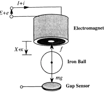
The structure of the electromagnetic suspension system is shown schematically in Fig- ure 3.1. The objective of our control experiments is to suspend an iron ball stably and firmly without any contact by controlling the attractive forces of an electromagnet. Note
that this system is essentially unstable.In Figure 3.1, a cylindrical electromagnet as an actuator is located at the upper part
34 CHAPTER3. ROBUSTCONTROLOFMAGNETICSUSPENSIONSYSTEMs
of the experimental system. Mass of the iron ball is 1.75 kg, and it has a diameter of 77
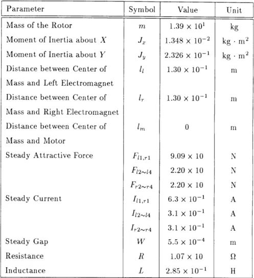
mm. A gap sensor of our own producing is placed at the bottom of the system to measure the gap length between the iron ball and the electromagnet. The sensor is scaled for a gap of 2.4 mm per volt. It is a standard induction probe of eddy-current type. Physical parameters of this experimental machine are shown in Table 3.1.
I+i
E+e
X+x ][
l'li x
x f
mg
k
Electromagnet
Iron Ball
Gap Sensor
Figure 3.1: Schematic diagram of the Electromagnetic Suspension System
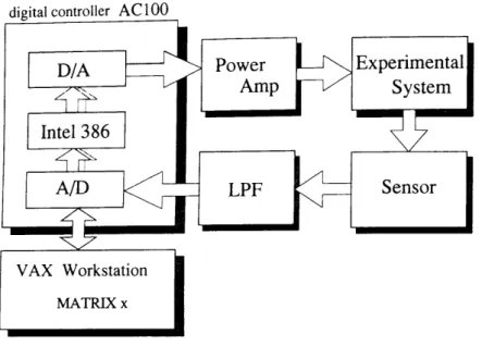
Digital Controller
The experimental machine is controlled by a digital controller using a DSP (Digital Signal
Processor). The experimental setup basically consists of the DSP which is sandwiched between A/D and D/A converters. Real-time control is implemented with a processor NEC paPD77`230, which can execute one instruction in 150 ns with 32-bit floating point
arithmetic. This device has enough fast processing speed to stabilize a relatively simple magnetic suspension system in Figure 3.1. The control algorithm is written in the assemblylanguage for the DSP and a software development is assisted by a host personal computer NEC PC-9801 under the MS-DOS environment. The data acquisition board MSP-77230 consist•s of a 12-bit A/D converter and a 12-bit D/A converter with the maximum conver-
sion speed of 10.5 pas and 1.5 pss, respectively.
The sensor outputs are filtered through an analog low-pass circuit, and then converted
to digital signals by A/D converters. The DSP calculates the control input signals. Thesedigital signals are converted to analog signals by D/A converters with a range of Å}5 V•
CHAPTER 3. ROBUST COIVTROL
The converted signals and the steady to actuate the electromagnet. Steady maximum voltage of a regulated DC
OF MAGNETIC SUSPENSION SYSTEMS 35
current signals are added and amplified by 10 times state voltage of the electromagnet is 24.6 V and the power supply is 70.0 V.
3.1.3 Model of Electromagnetic Suspension System
Our purpose in this section is to introduce an ideal mathematical model and an uncertainty
weighting function for the system. See [23] for details.Model Structures
We employ four different model structures for the system depicted in Figure 3.1. All of the models are finite-dimensional, linear, and time-invariant of the following state space form: