Comparison of numerical methods for 1‑D
hyperbolic‑type problems with free boundary
著者 ファイザル マホロス
著者別表示 Faizal Makhrus journal or
publication title
博士論文要旨Abstractおよび要約Outline 学位授与番号 13301甲第4315号
学位名 博士(理学)
学位授与年月日 2015‑09‑28
URL http://hdl.handle.net/2297/43822
Creative Commons : 表示 ‑ 非営利 ‑ 改変禁止
Dissertation Abstract
Comparison of numerical methods for 1-D hyperbolic-type problems with free boundary
1次元双曲型自由境界問題の数値解法の開発と評価
Graduate School of
Natural Science and Technology Kanazawa University
Major subject:
Division of Mathematical and Physical Sciences
Course:
Computational Science
School registration No.: 1223102012 Name: Faizal Makhrus
Chief advisor: Seiro OMATA
1 Introduction
In this thesis, we study hyperbolic-type problems with free boundary. The real case can be considered as a phenomenon of ”peeling tape attached to a surface”. From this phenomenon, we can obtain the energy function. This energy function can be derived into Euler-Lagrange equation. A previous research was conducted solving this equation using numerical method called fixed domain method and showed the high accuracy for its results [2]. However, this method only works when there is only one free boundary point.
On the other hand, this problem has been investigated before by adding smooth- ing characteristic function. We call this as approximated problem. It can be used to model droplet motion on a plane or bubble touching the water surface in higher dimension using numerical methods called discrete Morse flow. In this study, we want to investigate the accuracy of numerical methods solving the approximated problem. However, the exact solution is not available in all cases. Despite not hav- ing exact solution, we use the solution of fixed domain method to get the accuracy.
The numerical methods which we investigate are: two types of finite difference method, finite element method, and discrete Morse flow. In addition, we also in- vestigate the treatment in the free boundary to get optimal error and comparing two smoothing characteristic functions. Since the fixed domain method solutions are available in 1-D only, we consider 1-D problem in this study.
2 Physical model of peeling tape problem
In this section, we explain the phenomenon of peeling tape on a plane. Suppose there is a thin film adhered to a plane. We consider this film as our tape. It is peeled offfrom the plane and starts to expand along the sticked tape. The region where the tape is adhered is considered as a domainΩ. We assume that the tape has the same tension γ at any places. The shape of the tape is represented by a functionu : Ω →R. The shape ofu is obtained by measuring the energy of this phenomenon.
J(u)= Z τ
0
Z
Ω
γ
2|∇u|2− ρ
2u2tχu>0+ Q2 2 χu>0
dxdt. (1) We chooseγ =ρ=1. Letube the stationary point of (1) andu∈C0(Ω×(0, τ)∩ W1,2(Ω, τ)), then u satisfies
∆u−utt =0 in{u>0}. (2)
Moreover, ifu ∈C2(Ω×(0, τ)∩ {u > 0}) and∂{u > 0}is inC−1, thenuon the boundary satisfies
|∇u|2−u2t =Q2 on∂{u>0}. (3) We solve this Euler-Lagrange equation using fixed domain method.
Now we consider an approximation of (1) where the characteristic function is approximated using a smoothing characteristic function. Firstly, we define a smooth function calledβε(s).βε(s)∈C2(R), βε(s)≥0, and satisfies
βε(s)
=0 s≤0,
≤1/ε 0<s< εand|β0ε(s)| ≤ C ε2,
=0 ε≤ s.
It is also thatRε
0 βεds=1 and we defineBε Bε(u)=
Z u
0
βε(s)ds −→
ε→0
1 in{u>0}, 0 in{u=0},
which is the smoothing characteristic function ofχu>0. Then we rewrite the energy function
Jε(u)= Z τ
0
Z
Ω
1
2|∇u|2−χu>01
2u2t + Q2 2 Bε(u)
dxdt. (4) By taking the first variation of (4), our problem becomes
∆u−χu>0utt =−Q2
2 βε(u) inΩ×(0, τ), u(x,0)=u0(≥0)
ut =v0
u(x,t)|∂Ω= f(x,t) with f(x,0)=u0on∂Ω.
(5)
We will solve this problem using numerical methods above.
3 Numerical method
3.1 Explicit method 1 (spatial central difference + time forward dif- ference)
We represent equation (5) using explicit method withuxxapproximated by central difference. Supposeut =vthen
d
dtui(t)=vi(t), i=1, . . . ,N−1, χ{u>0}(xi,t)d
dtvi(t)= ui−1(t)−2ui(t)+ui+1(t) (∆x)2 − Q2
2(χε)0(ui(t)), i=1, . . . ,N−1.
(6) The initial and boundary conditions areu0(t) = f(t), u(0) = g(x), v0(t) = f0(t), andv(0)=h(x). We solve (6) using the 4th order Runge-Kutta.
3.2 Explicit method 2 (spatial and time central difference)
We approximateuxx andutt from equation (5) using central difference. [0, τ] is divided intoM, 0=t0<t1 < . . . <tM =τ.
χ{u>0}(xi,tk)uki+1−2uki +uk−i 1
(∆t)2 = uki+1−2uki +uki−1 (∆x)2 − Q2
2 (χε)0(uki), i=1, . . . ,N−1, and k=1, . . . ,M−1,
(7)
whereuki =u(xi,tk), i=0, . . . ,N. Then we calculate the solutions with following
χ{u>0}(xi,tk)uki+1=2uki −uk−1i +(∆t)2
uki+1−2uki +uki−1 (∆x)2 − Q2
2 (χε)0(uki)
. (8) The boundary conditions areu0(t)= f(t) andu(0)=g(x).
4 Finite Element Method
We take the weak form of equation (5) and define a test functionξ∈C∞0(Ω). Then we obtain
Z
Ω(χ{u>0}utt−uxx+ Q2
2 (χε)0(u))ξdx=0, ∀ξ ∈C∞0(Ω). (9)
We approximate solution asu(x,t)=PN
i=0ai(t)ϕi(x) whereϕiis basis function. The basis function is defined as
ϕi(x)=
x−xi−1
∆x xi−1≤ x≤ xi, xi+1−x
∆x xi≤ x≤ xi+1, 0, otherwise, i=1,2. . . . ,N−1.
Then by integration by parts (9) gives Z
Ω
χ{u>0}
N
X
i=0
(ai)ttϕi
ξ+
N
X
i=0
ai(ϕx)i
ξx+ Q2 2(χε)0(
N
X
i=0
aiϕi)ξ
dx=0,∀ξ ∈C∞0(Ω).
(10) We choose basis functionϕj;j=1, . . . ,N−1 as our test function and rewrite (10)
N
X
i=0
"
(ai)tt
Z
Ωχ{u>0}ϕiϕjdx
# +
N
X
i=0
"
(ai) Z
Ω(ϕx)i(ϕx)jdx
# +Q2
2 Z
Ω(χε)0(
N
X
i=0
aiϕi)ϕjdx=0 (11) j=1,2, . . . ,N−1
We change into matrix form
Batt+Aa+ Q2
2C(a)=0, (12)
wherea=a1, . . . ,aN−1,C is a column matrix whose elements are determined bya andbis determined by boundary values.
We approximateattusing central difference withak =a(x,tk).
Bak+1−2ak+ak−1
(∆t)2 +Aak+ Q2
2C(ak)=b. (13)
The final form is
Bak+1 =2Bak−Bak−1−(∆t)2
Aak+ Q2
2 C(ak)+b
. (14) We solve (14) using steepest decent method.
4.1 Discrete Morse Flow
Minimizing the functional below on function spaceκapproximates the weak solu- tion of equation (5) [1]
Jn(u)=Z
Ω
|u−2un−1+un−2|2
2(∆t)2 χ{u>0}dx+ 1 2
Z
Ω|∇u|2dx+ Q2 2
Z
Ωχε(u)dx. (15) κ={u∈W1,2(Ω);u=gon∂Ω}
Functionu0 andu1 are the approximate solutions at time levelt = 0 and t = ∆t respectively. We define the approximate solutionunfor the next time levelt=n∆t, n=2,3, . . . ,Nby minimizing (15).
5 Numerical Results
The initial conditions of our experiments are
l0= 1 pQ2+ f0(0)2 g(x)=max(1− 1
l0x,0), h(x)=
f0(0) 0< x≤l0, 0 l0< x, and f(t) are
case 1 Peeling speed is constant f(t) = at+1. The exact solution of this case is u(x,t)=max(1+t− 1
l0x,0).
case 2 Peeling speed is increasing f(t)=(at+1)2. case 3 Peeling speed is decreasing f(t)= √
at+1.
case 4 Peeling speed is stopping at some times f(t)=1+at+sin t
case 5 Peeling direction is downward (pasting the tape).
g(x)=max(10− 1 l0x,0), f(t)=10−at,
h(x)=
f0(0) 0<x≤l0, 0 l0 <x,
case 6 Peeling directions are upward and downward (oscillating tape) f(t) = 1+ 0.3 sin t.
5.1 The error of peeling tape model using smoothing characteristic function
The comparisons are shown in figures 1. From the figures, we can see that the errors of solutions from all cases tend to be small whendxis decreasing in some ε. They show that small and bigεgive big error.
In addition, the choice ofεto get minimum error also depends on the gradient of the solution near to free boundary point. To see this, we solve cases 1-4 with different gradients of solutions. We choose only cases 1-4 since they are enough to represent different kinds of solution. By changing parametera, the gradient of the solution can be set. We set the gradient vary from 2-40. We call this gradient asgu. The result is the appropriateεapproximately 8−360×dx.
(a)Eucase 1 at time levelτ=9 (b)Eucase 2 at time levelτ=9 Figure 1: errors of numerical solution of cases 1-6
5.2 Comparisons of smoothing characteristic functions
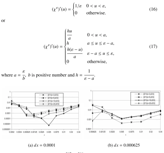
We compare two smoothing characteristic functions (16) and (17). We apply these two functions in equation (5) with some parametersQ2 = 1, Ω = [0,15], a = 1, dx=0.005, anddt=0.9dxand solve using explicit method 2.
(χε)0(u)=
1/ε 0<u< ε,
0 otherwise. (16)
or
(χε)0(u)=
hu
a 0<u<a, h a≤u≤ε−a,
h(ε−u)
a ε−a≤u≤ε,
0 otherwise,
(17)
wherea= ε
b, bis positive number andh= 1 ε−a.
(a)dx=0.0001 (b)dx=0.000625
Figure 2:|E˜17u −E˜16u |case 1 atτ=9
The comparisons in figure 2 is done by calculating|E˜17u − E˜u16| where ˜Eu17 is E˜uusing equation (17) (in figure 2 we callE f1) and ˜E17u is ˜Euusing equation (16) (in figure 2 we callE f2). From the figure, we can see that the error differences between two smoothing characteristic function are relatively similar that are in the order 10−3−10−4, if we considerεwhich are bigger 4−10×dx. Therefore, equation (16) is sufficient to be our smoothing characteristic function.
5.3 Comparisons of numerical methods
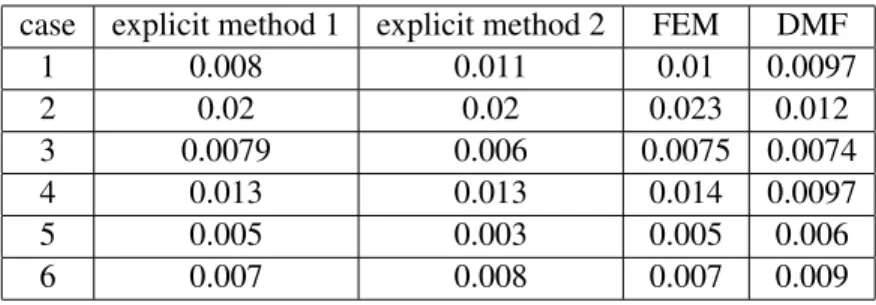
We compare four numerical methods by solving cases 1-6 and compare the errors of each methods. We choose the parametersQ2=1, Ω =[0,15], dx=0.005, ε= 0.04 anddt as in table 1. The errors of the methods are shown in table 2. Time complexity of each methods can be seen in table 3.
explicit method 1 explicit method 2 FEM DMF
0.9dx 0.9dx 0.5dx 0.1dx
Table 1:dtfor numerical methods
case explicit method 1 explicit method 2 FEM DMF
1 0.008 0.011 0.01 0.0097
2 0.02 0.02 0.023 0.012
3 0.0079 0.006 0.0075 0.0074
4 0.013 0.013 0.014 0.0097
5 0.005 0.003 0.005 0.006
6 0.007 0.008 0.007 0.009
Table 2:Euat timeτ=9 (cases 1-5) andτ=7 (case 6)
fixed domain method explicit method 1 explicit method 2 FEM DMF
time 2s 3s 3s 10mins >15mins
Table 3: Time complexity
The error differences of each numerical methods in table 2 are relatively small (order 10−3−10−4). Therefore, we conclude that all methods are good. However, based on the time complexity in table 3, DMF has big time complexity due to its algorithm and smalldt. On the other hand, DMF has advantage that it can be added some constraints such as volume constraint to support advanced model like droplet motion. Hence, this method is promising to be used further. We also try severaldt for DMF and we find that whendt=1/10dxthe errors of DMF solution approach the errors of other methods. In FEM, we find thatdt≤1/2dxgives stable solutions.
6 Conclusions
We solve 1D hyperbolic-type problem with free boundary and smoothing charac- teristic function by explicit method and compare with the exact or fixed domain method solutions. The results tell that the errors of explicit method depend on the selection of smoothing characteristic function parameterεanddx. In addition, the choice ofεdepends on the gradient of the solution. We also compare two kinds of smoothing characteristic functions and find that both have similar errors. Further- more, we compare four numerical methods solving the peeling tape problem and find that all methods have similar errors. However, based on time complexity, dis- crete Morse flow is the slowest. We also solve some cases where the free boundary points contains more than one points and they appear or vanish during simulation time. We obtain the solutions using four numerical methods and find that all of them give similar solutions. For the future research, it is interesting to implement this problem in higher dimensions.
References
[1] E. Ginder, K. Svadlenka,A variational approach to a constrained hyperbolic free boundary problem,Nonlinear Analysis 71 (2009) e1527-e1537
[2] H. Imai, K. Kikuchi, K. Nakane, S. Omata, T. Tachikawa, A numerical ap- proach to the Asymptotic Behavior of Solution of a one-dimensional free boundary problem of hyperbolic type, Japan J. of Ind. and Appl. Math. 18 (2001), 43 - 58.