Development of a semi-automatic measurement method for presampled MTF using virtual slit images

1

1．Introduction

 Photostimulable storage phosphor （PSP） and the flat panel detector （FPD） are used in a digital X-ray detector. The modulation transfer function （MTF） is used to evaluate the resolution property of the digital X-ray detector for quality assurance （QA） and quality control （QC） . The slit and edge methods are usually used to measure the MTF for the digital X-ray detector [1, 2]. The International Electrotechnical Commission

（IEC） recommends the edge method for digital X-ray detectors [3].

 The edge method uses an edge image of a slightly slanted tungsten edge device on the digital X-ray detector. The edge image is used to generate a composite oversampled edge spread function （ESF） , which is differentiated to obtain a synthesis line spread function （LSF） . Finally, the MTF is calculated by Fourier transform of the synthesis LSF. Although the edge method is simpler than the slit method, the former requires accurate measurement of the edge

angle from the edge image. The measurement error of the edge angle influences the accuracy of the MTF, so the edge angle is used to calculate the MTF. In addition, the edge method complicates the LSF generation process and requires a great deal of experience with its measurement. Many researchers were reported the precise of edge angles [5, 6].

 We previously proposed the “virtual slit” method, which uses an edge image [7]. The virtual slit method is a simplified MTF measurement process based on the edge method. Our original approach obtains a virtual slit image by subtracting the original edge image from the same image shifted one pixel in the horizontal direction. However, the virtual slit method has a problem in that the measurement error of the edge angle depends on a manual measurement process using ImageJ （National Institutes of Health, USA） [8].

The virtual slit method requires an accurate measurement of the edge angle because it is based on the edge method. For the virtual slit method, the

*Corresponding author. Tatsunori Kobayashi.

Tel.: +81 92-554-1244 Fax: +81 92-552-0072

E-mail: [email protected]

原著

Development of a semi-automatic measurement method

for presampled MTF using virtual slit images

Tatsunori Kobayashi, Yasuyuki Kawaji

Abstract: We have been researching the use of a virtual slit method on the presampled modulation transfer function

（MTF） . The virtual slit method obtains a virtual slit image by subtracting the edge image from an image shifted one pixel in the vertical direction. In our previous study, the measurement of the edge angle and synthesis of a line spread function

（LSF） were fully manual processes, which affected the MTF calculation error. The aim of the present study was developing semi-automatic software for the virtual slit method. We used four simulation edge images （edge angles: 1.5° , 2.0° , 2.5° , and 3.0°） and obtained three experimental edge images with an indirect flat panel detector. Our software can measure the edge angle, generate the LSF, and calculate the MTF semi-automatically. The measurement error of the edge angles was within 0.01° in all simulation images and within 0.02° in all experimental edge images, respectively. The error ratio of the simulated and theoretical MTFs was within 1.0% at the Nyquist frequency. The average standard deviation of the MTFs with the experimental edge images was within 0.0006 （maximum: 0.0013） . Thus, we developed semi- automatic software for the virtual slit method. Our results showed that the software can stably measure the MTF. We consider the software to be a useful semi-automatic assistant for the virtual slit method.

Key words: modulation transfer function, virtual slit image, edge angle, semi-automatically measurement

Department of Radiological Science, Faculty of Health Science, Junshin Gakuen University

純真学園大学雑誌 第9号 令和2年3月

Journal of Junshin Gakuen University，

Faculty of Health Sciences Vol.9， March 2020

2 Tatsunori Kobayashi, Yasuyuki Kawaji

measurement error of the edge angle has to be reduced to improve the MTF calculation accuracy.

Therefore, we developed software that semi- automatically measures the MTF by using the virtual slit method. The purpose of this study was to develop a semi-automatic method to reduce the measurement error from manual processes. Our software can measure the edge angle, generate the synthesis LSF, and calculate the MTF semi-automatically. In this paper, we discuss the accuracy of the edge angle and MTF with the proposed method and describe the usefulness of our software.

2

Materials and methods 2.1. Simulation edge image

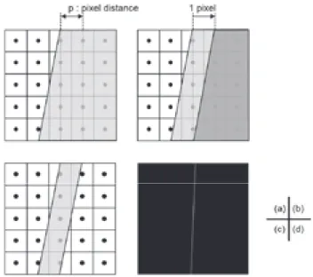
 We simulated images by using a Lorentzian-shaped function [6]. The simulation images had a matrix size of 65×512 pixels, gray-level resolution of 16 bits, and sampling pitch of 0.0875 mm/pixel. The Nyquist frequency （Ny） was 5.71 cycles/mm. Figure 1 shows four simulation images with edge angles of 1.5° , 2.0° , 2.5° , and 3.0° .

Fig. 1　Simulation images with edge angles of （a） 1.5°,

（b） 2.0°, （c） 2.5°, and （d） 3.0°.

4

the edge angle and MTF with the proposed method and describe the usefulness of our software.

67 68

2. Materials and methods 69

2.1. Simulation edge image 70

We simulated images by using a Lorentzian-shaped function [6]. The simulation images had a 71

matrix size of 65 × 512 pixels, gray-level resolution of 16 bits, and sampling pitch of 0.0875 72

mm/pixel. The Nyquist frequency (Ny) was 5.71 cycles/mm. Figure 1 shows four simulation images 73

with edge angles of 1.5°, 2.0°, 2.5°, and 3.0°.

74

Fig. 1 Simulation images with edge angles of (a) 1.5°, (b) 2.0°, (c) 2.5°, and (d) 3.0°.

2.2. Experimental measurements

 We used three experimental edge images that were the same as those used in our previous study [7].

These images were obtained with an indirect FPD detector （PLAUDR, Konica Minolta, Tokyo, Japan）

and the tungsten edge device. The FPD was implemented with a CsI-based phosphor. We removed the X-ray scatter reduction grid and disabled all image processing. The RQA5 spectrum was used for all measurements by adding 21 mm of aluminum to a 74 kV X-ray beam to provide an approximate half-value layer of 7.1 mm of Al. The experimental edge images had a matrix size of 1K × 1K pixels, resolution of 16 bits, and sampling pitch of 0.139 mm/pixel. Ny of the edge images was 3.60 cycles/mm. The tungsten edge device was slightly slanted at 1.5 ° -3 ° relative to the vertical direction of the pixel matrix on the FPD. Our software used a region of interest （ROI） image with a matrix size of 768 × 512 pixels from the experimental edge image to measure the MTF. Figure 2 shows an example ROI image with the tungsten edge device on the right side.

Fig. 2　Example ROI image obtained from the experimental edge image. The right side shows the tungsten edge device with a slight angle.

5 75

2.2. Experimental measurements 76

We used three experimental edge images that were the same as those used in our previous study 77

[7]. These images were obtained with an indirect FPD detector (PLAUDR, Konica Minolta, Tokyo, 78

Japan) and the tungsten edge device. The FPD was implemented with a CsI-based phosphor. We 79

removed the X-ray scatter reduction grid and disabled all image processing. The RQA5 spectrum 80

was used for all measurements by adding 21 mm of aluminum to a 74 kV X-ray beam to provide an 81

approximate half-value layer of 7.1 mm of Al. The experimental edge images had a matrix size of 82

1K × 1K pixels, resolution of 16 bits, and sampling pitch of 0.139 mm/pixel. Ny of the edge images 83

was 3.60 cycles/mm. The tungsten edge device was slightly slanted at 1.5°-3° relative to the vertical 84

direction of the pixel matrix on the FPD. Our software used a region of interest (ROI) image with a 85

matrix size of 768 × 512 pixels from the experimental edge image to measure the MTF. Figure 2 86

shows an example ROI image with the tungsten edge device on the right side.

87

Fig. 2 Example ROI image obtained from the experimental edge image. The right side shows the tungsten edge

2.3. Semi-automatic processing

Figures 3 （a） and （b） show fl owcharts comparing the

processes of our previous study and our software. The

dotted lines in Fig. 3 （b） indicate the semi-automated

process in our software.

3 Development of a semi-automatic measurement method for presampled MTF using virtual slit images

Fig. 3　Comparison of the process fl ows in the previous study and with the semi-automatic MTF calculation software: （a） fl owchart of the previous study [7] and

（b） fl owchart of our semi-automatic method. 6

device with a slight angle.

2.3. Semi-automatic processing 88

Figures 3a and b show flowcharts comparing the processes of our previous study and our software.

89

The dotted lines in Fig. 3b indicate the semi-automated process in our software.

90

Fig. 3 Comparison of the process flows in the previous study and with the semi-automatic MTF calculation software:

2.4. Dose image

 A pixel is a saved digital value in a digital image obtained by using FPD. We can convert the digital value （DV

） into the dose value （d

） in each pixel by using Eq. （1） on the measurement MTF:

 d

= a × e

（1）

where a and b are coefficients obtained from the digital characteristic curve and DVmax is the maximum digital value in the ROI image. In this study, a was 1.058, and b was 0.014.

2.5. Virtual slit image

 Here, we describe the generation of the virtual slit image in Fig. 4. First, we shift the dose image by one

pixel in the horizontal direction, as shown in Figs. 4

（a） and （b） . The virtual slit image is obtained by subtracting the dose image from the shifted image, as shown in Fig. 4 （c） . Figure 4 （d） shows an example virtual slit image of the experimental edge image.

Fig. 4 Generation of a virtual slit image: （a） schematic diagram of a dose image, （b） shifted image generated by moving the dose image by one pixel to the horizontal direction, （c） subtraction image obtained by subtracting the dose image from the shifted image, and （d） example virtual slit image in the experiment.

8

Fig. 4 Generation of a virtual slit image: (a) schematic diagram of a dose image,

(b) shifted image generated by moving the dose image by one pixel to the horizontal direction, (c) subtraction image obtained by subtracting the dose image from the shifted image, and (d) example virtual slit image in the experiment.

103

2.6. Measurement of the edge angle 104

Our proposed method measures the edge angle by using the maximum pixel in each row of the 105

virtual slit image. Our software can objectively measure the edge angle by using the maximum 106

image. The maximum image is obtained by extracting the maximum value of each row in the virtual 107

slit image, as shown in Fig. 5a. The maximum pixels are continuous in the maximum image, as 108

shown in Fig. 5b. Thus, we extract the maximum pixel value from the continuous maximum pixels, 109

as shown in Fig. 5c. The edge angle is calculated by using the x-axis and y-axis coordinates of the 110

discrete maximum pixel value in the maximum image. The edge angle is calculated as follows:

111

2.6. Measurement of the edge angle

 Our proposed method measures the edge angle by using the maximum pixel in each row of the virtual slit image. Our software can objectively measure the edge angle by using the maximum image. The maximum image is obtained by extracting the maximum value of each row in the virtual slit image, as shown in Fig. 5a.

The maximum pixels are continuous in the maximum image, as shown in Fig. 5b. Thus, we extract the maximum pixel value from the continuous maximum pixels, as shown in Fig. 5c. The edge angle is calculated by using the x -axis and y -axis coordinates of the discrete maximum pixel value in the maximum image. The edge angle is calculated as follows:

 α = tan （

_x ^y

^y

lower

x

） ^（2）

where x

and y

are the x- and y-axis coordinates

for the upper row, and x

and y

are the x- and

4 Tatsunori Kobayashi, Yasuyuki Kawaji

y-axis coordinates for the lower row in the maximum image, as shown in Fig. 5 （d） .

Fig. 5　Calculation of the edge angle using the maximum image: （a） maximum pixel values of each row in the virtual slit image, （b） maximum pixel value in each sequential column of the maximum pixel value, as shown in Fig. 3（a）, and （c） edge angle calculated from the coordinate information for the maximum pixel value in the upper and lower rows of the maximum image.

9 𝛼𝛼𝛼𝛼= tan⁻¹�^{𝑦𝑦𝑦𝑦}𝑢𝑢𝑢𝑢𝑢𝑢𝑢𝑢𝑢𝑢𝑢𝑢𝑢𝑢𝑢𝑢𝑢𝑢𝑢𝑢 − 𝑦𝑦𝑦𝑦𝑙𝑙𝑙𝑙𝑙𝑙𝑙𝑙𝑙𝑙𝑙𝑙𝑢𝑢𝑢𝑢𝑢𝑢𝑢𝑢

𝑥𝑥𝑥𝑥𝑙𝑙𝑙𝑙𝑙𝑙𝑙𝑙𝑙𝑙𝑙𝑙𝑢𝑢𝑢𝑢𝑢𝑢𝑢𝑢 − 𝑥𝑥𝑥𝑥𝑢𝑢𝑢𝑢𝑢𝑢𝑢𝑢𝑢𝑢𝑢𝑢𝑢𝑢𝑢𝑢𝑢𝑢𝑢𝑢� (2)

112

where xupper and yupper are the x- and y-axis coordinates for the upper row, and xlower and ylower are the 113

x- and y-axis coordinates for the lower row in the maximum image, as shown in Fig. 5d.

114

Fig. 5 Calculation of the edge angle using the maximum image: (a) maximum pixel values of each row in the virtual slit image, (b) maximum pixel value in each sequential column of the maximum pixel value, as shown in Fig. 3(a), and (c) edge angle calculated from the coordinate information for the maximum pixel value in the upper and lower rows of the maximum image.

115

2.7. Calculation of the integer number N 116

The edge method uses the integer number N to generate the synthesis LSF [8]. We obtain the N as 117

follows:

118

𝑁𝑁𝑁𝑁=_{tan 𝛼𝛼𝛼𝛼}^1.0 (3)

119

2.7. Calculation of the integer number N

 The edge method uses the integer number N to generate the synthesis LSF [8]. We obtain the N as follows:

 N = 1.0

tan α （3）

where α is the edge angle.

2.8. Generation of the synthesis LSF

 Our software extracts an ROI with ±2N rows around the center y-coordinate to measure the MTF in the virtual slit image, as shown in Fig. 6 （a） . We can obtain the synthesis LSF by repositioning the pixels within the ROI in the virtual slit image [1], as shown in Fig. 6 （b） .

Fig. 6　Generation of a synthesis LSF: （a） ROI region of N rows extracted from the virtual slit image and

（b） synthesis LSF obtained from repositioning the pixels in the ROI from Fig. 6（a）.

10 where α is the edge angle.

120 121

2.8. Generation of the synthesis LSF 122

Our software extracts an ROI with ±2N rows around the center y-coordinate to measure the MTF 123

in the virtual slit image, as shown in Fig. 6a. We can obtain the synthesis LSF by repositioning the 124

pixels within the ROI in the virtual slit image [1], as shown in Fig. 6b.

125

Fig. 6 Generation of a synthesis LSF: (a) ROI region of N rows extracted from the virtual slit image and (b) synthesis LSF obtained from repositioning the pixels in the ROI from Fig. 6(a).

126

2.9. Generation of averaged synthesis LSF 127

We use three synthesis LSFs to calculate an MTF. The maximum value positions are different for 128

each synthesis LSF as shown in Fig. 7a. To obtain the averaged synthesis LSF as shown in Fig. 7b, 129

the peak coincides with each synthesis LSF, and the average value of these LSFs is calculated. We 130

verify the peak of each synthesis LSF using the Excel spreadsheet application (Microsoft 131

Corporation, Redmond, WA, USA).

132

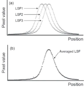
2.9. Generation of averaged synthesis LSF

 We use three synthesis LSFs to calculate an MTF.

The maximum value positions are different for each synthesis LSF as shown in Fig. 7a. To obtain the averaged synthesis LSF as shown in Fig. 7b, the peak coincides with each synthesis LSF, and the average value of these LSFs is calculated. We verify the peak of each synthesis LSF using the Excel spreadsheet application （Microsoft Corporation, Redmond, WA, USA） .

Fig. 7　Generation of the averaged synthesis LSF: （a）

the positions of maximum value are diff erent in each synthesis LSF; （b） the positions of the maximum pixel values are repositioned to coincide with the maximum pixel value position in each LSF to obtain the averaged LSF.

11

Fig. 7 Generation of the averaged synthesis LSF: (a) the positions of maximum value are different in each synthesis LSF; (b) the positions of the maximum pixel values are repositioned to coincide with the maximum pixel value position in each LSF to obtain the averaged LSF.

133

2.10. Calculation of the resampled MTF 134

The presampled MTF (MTFo) is obtained by using discrete Fourier transform (DFT) on the 135

synthesis LSF. We correct the presampled MTF(MTFp) with the sinc function as follows [9]:

136

𝑀𝑀𝑀𝑀𝑀𝑀𝑀𝑀𝑀𝑀𝑀𝑀𝑝𝑝𝑝𝑝= 𝑀𝑀𝑀𝑀𝑀𝑀𝑀𝑀𝑀𝑀𝑀𝑀𝑙𝑙𝑙𝑙 sin (𝑓𝑓𝑓𝑓𝑓𝑓𝑓𝑓𝑓𝑓𝑐𝑐𝑐𝑐𝑙𝑙𝑙𝑙𝑐𝑐𝑐𝑐𝑐𝑐𝑐𝑐𝑓𝑐𝑐𝑐𝑐)

(𝑓𝑓𝑓𝑓𝑓𝑓𝑓𝑓𝑓𝑓𝑐𝑐𝑐𝑐𝑙𝑙𝑙𝑙𝑐𝑐𝑐𝑐𝑐𝑐𝑐𝑐𝑓𝑐𝑐𝑐𝑐)

(4) 137

where f is the spatial frequency, α is the edge angle, and s is the sampling pitch of the input image． 138

139 140

5 Development of a semi-automatic measurement method for presampled MTF using virtual slit images

2.10. Calculation of the resampled MTF

 The presampled MTF （MTF

） is obtained by using discrete Fourier transform （DFT） on the synthesis LSF. We correct the presampled MTF（MTF

） with the sinc function as follows [9]:

 MTF

= MTF

sin（f･π･cosα･s）

       （f･π･cosα･s）

（4）

where f is the spatial frequency, α is the edge angle, and s is the sampling pitch of the input image．

2.11. Calculation of the theoretical MTF

 The theoretical MTF of the edge image can be analytically computed and is given by a Lorentzian- type function. The theoretical MTF （MTFt） is calculated by using Eq. （5） [8] and then corrected by the sinc function [9]. Equation （5） uses the regular subsampling pitch given by the lateral distance between two adjacent pixels p divided by the number of lines N corresponding to a lateral shift of the edge by one pixel:

 MTFt = r

r

+ （2πf）

× sin （f･π･cosα･s）

（f･π･cosα･s） （5）

where r is the value of （1/p） for the edge parameter, as shown in Fig. 4a, f is the spatial frequency, α is the edge angle, and s is the sampling pitch of the input image.

2.12. Calculation of the error ratio of MTF

We can calculate the error ratio between the MTF of the simulation images （MTFsi） and MTFt by using Eq. （6） to estimate the accuracy of MTFsi.

 error ratio = MTF

MTF

MTF

× 100 （6）

3．Results

3.1. Measurement of the edge angle in simulation images

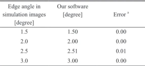
 We measured the edge angles in simulation edge images by using Eq. （2） , and the results are presented in the second column of Table 1. We calculated the errors between the edge angle of the simulation images and our results to estimate the accuracy of our method.

The measured edge angle in the simulation images is presented in the third column on of Table 1. The measurement error of the edge angle was within 0.01°

for all of the simulation images.

Table 1　Edge angles measured by our software in four simulation images

Edge angle in simulation images

[degree]

Our software

[degree] Error ^a

1.5 1.50 0.00

2.0 2.00 0.00

2.5 2.51 0.01

3.0 3.00 0.00

a = error is between our software and the average of the manual measurement

3.2. Measurement of the edge angle in experimental edge images

 We measured the edge angles in the experimental edge images by using Eq. （2） , and the results are presented in the first column of Table 2. The edge angle was manually measured by two radiological technologists （RTs） independently, and the results are presented in the second and third columns of Table 2.

The maximum error was 0.04 by RT1, and the minimum error was 0.01. We calculated the average edge angle of each experimental edge image by the two RTs. We calculate the errors between the averaged and semi- automatically measured results to estimate the accuracy of our method. The measurement error of the edge angle was within 0.02° for all of the experimental edge images.

Table 2　Comparison between the edge angles with our software and manual measurement in three experimental edge images

Image number

Our software [degree]

Manual measurement [degree] (error^a)

RT1 RT2 Average

1 2.32 2.35 (0.03) 2.31 (-0.01) 2.33 (0.01) 2 2.32 2.36 (0.04) 2.31 (-0.01) 2.34 (0.02) 3 2.32 2.35 (0.03) 2.31 (-0.01) 2.33 (0.01) a= error is between our results and the average of the manual measurement RT= radiological technologist

3.3. Presampled MTFs of the simulation image

Figure 8 （a） - （d） compares the simulation and

theoretical MTFs. The error ratio of these MTFs was

within 1.0% （at Ny/2 and Ny） , as given in Table 3.

6 Tatsunori Kobayashi, Yasuyuki Kawaji

14

Fig. 8 Comparison between the MTFs of four simulation images and the theoretical values. The MTF with edge angles of (a) 1.5°, (b) 2.0°, (c) 2.5°, and (d) 3.0°.

183

Table 3 Comparison between the error ratios of the MTFs in four simulation edge images Edge angle of simulation

image [degree] error ratio [%]

at Ny/2 error ratio [%]

at Ny

1.5 -0.03 -0.17

2.0 -0.05 -0.68

2.5 0.05 -0.07

3.0 0.04 -0.02

Ny = Nyquist frequency, Ny/2 = Half of the Nyquist frequency 184

3.4. Presampled MTF of the experimental edge image 185

Figure 9a-c compares three MTFs of the experimental image and the averaged MTF of the three 186

Fig. 8　Comparison between the MTFs of four simulation images and the theoretical values. The MTF with edge angles of （a） 1.5°, （b） 2.0°, （c） 2.5°, and （d）

3.0°.

Table 3　Comparison between the error ratios of the MTFs in four simulation edge images

Edge angle of simulation image [degree]

error ratio [%]

at Ny/2 error ratio [%]

at Ny

1.5 -0.03 -0.17

2.0 -0.05 -0.68

2.5 0.05 -0.07

3.0 0.04 -0.02

Ny = Nyquist frequency, Ny/2 = Half of the Nyquist frequency

3.4. Presampled MTF of the experimental edge image

 Figure 9 （a） - （c） compares three MTFs of the experimental image and the averaged MTF of the three MTFs. The averaged standard deviation （SD） was 0.0006 （maximum: 0.0013） among the three MTFs.

4．Discussion

 We developed a semi-automatic measurement software for the virtual slit method to realize accurate measurement of the edge angle. The edge angle affects the accurate calculation of the MTF because it is used to calculate N in Eq. （3） . Therefore, evaluating the accuracy of the edge angle measurement with our software was important.

 In our previous study, the edge angle was measured through a manual process [7]. In this study, our proposed method can semi-automatically measure the

edge angle by using the coordinates of the maximum pixel in the edge image. This approach can reduce the subjective error depending on the manual process and assure a reproducible measurement of the edge angle.

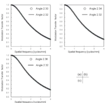
The measurement results of our software matched the edge angles in the simulation images and experimental edge images, as given in Tables 1 and 2. The maximum error of the edge angle was 0.02° . We calculated the MTFs for edge angles of 2.30° , 2.34° , and 2.36° and compared them with an MTF for an edge angle of 2.32° , as shown in Fig. 10. The fi rst three MTFs approximately coincided with the last MTF, and the SD for the four MTFs was 7.5 × 10

. We concluded that the error of the edge angle did not infl uence the calculation of the MTF and that our software can accurately measure the edge angle.

The SD of the MTFs for the simulation images was within 1.0% （at Ny/2 and Ny） , as given in Table 3 and Fig. 8. The results showed that our method can approximate the theoretical MTF. The maximum error ratio of our result was -0.68 at 2° in the simulation image. In Bhur et al.ʼs study, the error was within 1.0%

at 2° in simulation images [6]. Our proposed method can reduce the relative error of the MTF in simulation images.

15

MTFs. The averaged standard deviation (SD) was 0.0006 (maximum: 0.0013) among the three 187

MTFs.

188

Fig. 9 Comparison between MTFs of three FPD images and the average value. The MTF with (a) edge image 1, (b) edge image 2, and (c) edge image 3.

189

4. Discussion 190

We developed a semi-automatic measurement software for the virtual slit method to realize 191

accurate measurement of the edge angle. The edge angle affects the accurate calculation of the MTF 192

because it is used to calculate N in Eq. (3). Therefore, evaluating the accuracy of the edge angle 193

measurement with our software was important.

194

Fig. 9　Comparison between MTFs of three FPD images

and the average value. The MTF with （a） edge

image 1, （b） edge image 2, and （c） edge image 3.

7 Development of a semi-automatic measurement method for presampled MTF using virtual slit images

17

Fig. 10 Comparison between MTFs with edge angles of 2.32°and (a)2.30°, (b)2.34°, and (c)2.36° in experimental edge image 2.

210

For the simulation image with an edge angle of 2.0°, the error was higher than in other simulation 211

images. This error may have been due to the N value used to generate the synthesis LSF. Although 212

we obtained a true N of 28.59 with Eq. (3), our method used the integer N of 29 in the semi- 213

automatic process. The difference between the true N and integer N affected the accuracy when the 214

synthesis LSF was generated. Further investigation is needed to reduce the influence of the error 215

between the integer N and true N on the virtual slit image.

216

The averaged SD of the MTFs in the experimental edge images were within 0.0006 (maximum:

217

Fig. 10　Comparison between MTFs with edge angles of 2.32° and （a）2.30°, （b）2.34°, and （c）2.36° in experimental edge image 2.

 For the simulation image with an edge angle of 2.0° , the error was higher than in other simulation images.

This error may have been due to the N value used to generate the synthesis LSF. Although we obtained a true N of 28.59 with Eq. （3） , our method used the integer N of 29 in the semi-automatic process. The difference between the true N and integer N affected the accuracy when the synthesis LSF was generated.

Further investigation is needed to reduce the infl uence of the error between the integer N and true N on the virtual slit image.

 The averaged SD of the MTFs in the experimental edge images were within 0.0006 （maximum: 0.0013） , and the MTFs coincided in value for the three images, as shown in Fig. 9. Our edge measurement method can measure the edge angle accurately and objectively because it uses the coordinates of the maximum pixel for the edge angle. Our proposed method can reduce the subjective error of the edge angle due to manual measurement and improve the reproducibility of the MTF. The results showed that our method can help with realizing stable and highly reproducible measurement of the MTF for edge images. We consider our results useful for MTF measurement in QA and QC of digital X-ray detectors.

 In addition, our method can freely set parameters for the sampling pitch, digital coefficient of the characteristic curve, and edge angle. The features of our method can be used for detailed analysis of the influence of each parameter during the MTF measurement process and will be the subject of future research.

 Currently, our software is Character user interface with the command line tool, and we require ImageJ and spreadsheet to confirm our output data. We will develop a graphical user interface to upgrade usability.

5．Conclusion

 We developed a semi-automatic measurement software to assist with presampled MTFs using virtual slit images. The results show that our software can accurately measure the edge angle and stably calculate the MTF. Further research is to develop an automatically generate the averaged synthesis LSF from some synthesis LSFs. Therefore, this software is useful for measuring the MTF when using a virtual slit image.

Acknowledgments

 We are grateful to Dr. Fukai Tyofuku and Dr Hiroshi Fujita.

Confl ict of interest

 The authors have no confl icts of interest to declare.

Reference

1．Fujita H, Doi K, Giger ML. Investigation of Basic Imaging Properties in Digital Radiography. 6. MTFs in II-TV Digital Imaging Systems. Med Phys. 1985 ; 12（6） :713-20.

2．Fujita H, Tsai DY, Itoh T, Doi K, Morishita J, Ueda K, Ohtsuka A. A simple method for determining the modulation transfer function in digital radiography. IEEE Trans Med Imaging. 1992 ; 11 : 34-9.

3 ．Samei E, Ranger NT, Dobbins JT 3rd, Chen Y.

Intercomparison of methods for image quality characterization. I. Modulation transfer function. Med Phys. 2006 ; 33 : 1454-65.

4．IEC 62220-1. Medical electrical equipment-Characteristics

of digital X-ray imaging devices Part 1: Determination of

8

the detective quantum efficiency, ed. 1.0, 2003.

5．Kawashita I, Maeda K, Arimura H, Morikawa K, Ishida T.

Development of an automated method for evaluation of sharpness of digital radiographs using edge method 6．Higashide R, Ichikawa K, Kunitomo H, Ohashi K, Kawano

M. Influence of angle-measurement error on pre-sampled MTF and proposal of an optimal technique of angle measurement, Nippon Hoshasen Gijutsu Gakkai Zasshi 65

（2） : 245-53, 2009.

7．Kawaji Y, Toyofuku F. A new simplified practical method for measuring the presampled MTF of digital radiographic systems using an edge device. The 6th JKMP and the 11th AOCMP Meeting proceedings. 2011 sep.29-30. CD-R.

8．Rasband WS. ImageJ, U.S. National Institutes of Health, Bethesda, Maryland, USA, imagej.nih.gov/ij/, 1997-2016.

9．Buhr E, Gu¨nther-Kohfahl S, Neitzel U. Accuracy of a simple method for deriving the presampled modulation transfer function of a digital radiographic system from an edge image. Med Phys. 2003 ; 30 : 2323-31.

10. Cunningham IA, Fenster A. A method for modulation transfer function determination from edge profiles with correction for finite-element differentiation. Med Phys.

1987 ; 14 : 533-7.