Net Buyers and Sellers of Labor: Linkage Between Monetary and Time Inequality

Net Buyers and Sellers of Labor:

Linkage Between Monetary and Time Inequality

Dimitry Rtischev

ABSTRACT

Consumption of products and services involves paying for other peopleʼs labor. Since everyone is endowed with 24 hours per day but works and consumes differently, there must exist net sellers and net buyers of time. We theoretically explore the equilibrium pattern of net selling and buying of time in an economy of agents with unequal wealth endowments. After demonstrating how trade in time reduces inequality in wealth but creates inequality in time, we discuss implications and extensions.

Keywords: labor supply, labor demand, leisure, inequality JEL classification: D31, J22, J23

1. Introduction

Consider a trucker and a lawyer, each of whom works, say, 10 hours a day. Although both sell the same amount of personal time for a wage, the typical lawyer earns and spends much more than the typical trucker. In particular, the lawyer spends more on gardeners, cleaners, tutors, counselors, trainers, accountants, entertainers, restaurants, airplanes, and hotels, not to mention manufactured goods whose production and distribution involves the work of many people he never sees. Moreover, the lawyerʼs wife and children, who also consume many hours of othersʼ labor, probably work fewer hours if at all, compared to the truckerʼs wife and children. All of this makes the lawyer and his household net buyers of other peopleʼs labor, and the trucker and family, net sellers. In other words, the lawyer, in effect, has more than 24 hours of human time per day at his disposal, whereas the trucker makes do with less than 24.

Since everyone is endowed with 24 hours per day but works and consumes differently, people (or households) that comprise an economy can be classified as net sellers of time, net buyers of time, or balanced traders of time. It would be an interesting but difficult exercise to obtain an empirical picture of the economy in terms of these classes. This paper makes an analytical attempt using a simplistic but

＊） Faculty of Economics, Gakushuin University, Tokyo. I thank Chan-Hyun Sohn for comments on an earlier version of this paper.

revealing framework. We frame the issue in terms of two goods, one equally distributed among all agents (e.g., time) and another (e.g., wealth, income) distributed unequally. We then allow agents to trade and examine the post-trade distribution of the two goods and the market-clearing price.

Modern work on the allocation of time builds on Beckerʼs (1965) seminal model. Beckerʼs key insight was to treat time outside of paid employment together with goods and services bought by a household as an essential input into a process which generates the utility that the household ultimately enjoys. Gronau (1977) extended Beckerʼs model by disaggregating time outside of paid employment into time spent on leisure and unpleasant “home work” (e.g., cleaning). But neither Becker nor Gronau explicitly considered the time of others that a household buys as part of its purchase of goods and services, and how such “bought time” compares to the “sold time” the household supplies on the labor market. One place where these issues do come up is in the literature that applies the general time allocation models to agricultural households, since buying and selling farm labor is both important and observable in the case of family farms. (Barnum and Squire, 1979) But although the agricultural household models explicitly consider both bought and sold labor, they mostly focus on the representative household and do not pursue the patterns of net exchange in labor among the households.

In Veblenʼs (1899/2007) model of the economy, the “leisure class” ostentatiously abstained from work, relying entirely on buying other peopleʼs time. Linder (1970) shifted attention from the ultra-rich to the more numerous “harried leisure class,” namely people who sell time as high-wage specialists and use part of the income to buy help in the services sector staffed by the working poor. Although the balance of trade in labor time across classes is an underlying theme in these writings, it does not receive explicit treatment.

The empirical literature on householdsʼ labor supply and leisure also does little to inquire into the net buying or selling of time. Aguiar and Hurst (2007) examined work and leisure trends in the US over five decades and reported, among other findings, that the more-educated, higher-paid workers have increased their paid working hours since the 1970ʼs, while the less-educated, lower-paid workers have curtailed theirs. McGrattan and Rogerson (2004) also report reallocation of paid employment hours in the US from males to females, from older to younger people, and from single- to married-person households.

Confining attention to changes in the hours of labor sold by representative members of various groups, these papers do not consider the changes in the number of workers in those groups and how much labor is included in the products and services they consume. Without inquiring into how the population ratio of lower-paid workers to higher-paid workers has changed, we cannot rule out the possibility that the higher-paid workers are buying and benefitting from more hours of other peopleʼs labor than the additional hours they themselves are spending in the office.

Several recent books meticulously document the bifurcation of the American economy over the past several decades into a well-educated, well-paid minority and a lower-wage, less-educated majority.

(Florida 2011, Murray 2013, Temin 2017). The books note that representative members of the well-paid

minority work longer hours than representative members of the lower-wage majority, but neglect to

examine the situation from the perspective of trade in time. Yet it is trade in time that enables the

professionals to pursue their intensive careers and intensive leisure activities. Comparing the classes not

only in terms hours of own labor sold but also in terms of hours of othersʼ labor bought may reveal a

very different picture. Rather than seeing the situation as that of a hard-working upper class and a hardly working lower class, the view that is likely to emerge from a net-trade-in-time analysis is that of a representative member of the upper class with much more than 24 hours of human time per day at his disposal and a representative member of the lower class with less than 24.

Without prior models to build upon, our goal will be to get a sense of the issues at stake using as simple a model as possible.

The next section presents the general model, followed by three sections which solve the model for a particular utility function and three kinds of initial wealth distributions.

Section 6 considers extensions and Section 7 concludes.

2. Model

There is a unit mass of agents uniformly distributed on the unit interval. Each agent i ∈ [0, 1] is endowed with T units of an “equal” good and w(i) units of a “variable” good. Until we discuss extensions, we will refer to the equal good as “time,” in the sense that everyone is endowed with 24 hours per day, and to the variable good as “wealth” or “money.”

The initial wealth distribution satisfies w(i) > 0 and wʼ(i) ≤ 0, ∀i ∈ [0, 1]. Thus, we order richer agents to be to the left of poorer agents.

Agents derive utility from both time and money. The more money and time the better, but each additional hour or dollar brings less utility than the previous one. Specifically, each agent has the same utility function u(t, m) whose derivatives satisfy u

> 0, u

< 0, u

> 0, u

< 0. Agent iʼs initial utility is u(T, w(i)).

Agents can exchange any amount of time for any amount of money within limits of their endowments.

There is no credit or savings. The market is organized well so that there is a single price p defined as money per hour. Let x(i) denote the net time bought or sold by agent i. If positive, the agent is a net buyer of time from other agents. If negative, the agent is a net seller of time to other agents. Post-trade, agent i has m(i) = w(i) − px(i) in money he can spend on consumption of goods, has t(i) = T + x(i) hours of own and (possibly) otherʼs labor at his disposal, and obtains utility u(t(i), m(i)).

Each agent is one of: a net seller of time to others, net buyer of time from others, balanced buyer and seller of time, or abstainer. Although each buyer can buy time from several sellers and each seller can sell time to several buyers, the number of sellers or buyers interacting with each buyer or seller is not of interest in our model. Likewise, we do not distinguish an agent who abstains from trade from an agent who buys and sells the same number of hours.

Definition. An equilibrium is a price p and transactions x(i) such that no agent can increase his utility by changing his transactions, the market clears, and all agentsʼ time and money budget constraints are met. That is, in equilibrium

1） A literature search for “net seller (buyer) of time” and “net seller (buyer) of labor (labour)” did not turn up any papers focused on the issues that we pursue.

1

0

x(i)di = 0       (1)

x(i) >− T i [0, 1]       (2) px(i) ≤w(i) i [0, 1]       (3) u(T＋x(i), w(i)

∀x’≠x(i), x’ ≥−T, px’≤w(i)

      (4) A necessary condition for an interior equilibrium is equality of the price of time to the marginal rate of substitution between time and money:

u

u

= p       (5) We will use the Gini coefficient to compare inequality in pre- and post-trade distributions of wealth as well as in post-trade distribution of time. The Lorenz curve (fraction of wealth owned by the poorest fraction q of the population) is

L(q) = 1 W

w(1−i)di

0

       (6) where W = w(i)di

is the total wealth in the population. The Gini coefficient (area between the diagonal and the Lorenz curve divided by the area of the triangle below the diagonal) is

g = 2    (q−L(q))dq = 1− 2 w(1−i)didq W

q 0 1 0 1

0

      (7)

When using the above formulas to compute the Gini coefficient for ex-post wealth and time, we will use m(i) and t(i) in place of w(i), respectively.

3. A two-class economy

Let us first examine the simplest case: a population with two types of agents. A fraction k of the population consists of “rich” agents each of whom is endowed with wealth a. The rest of the population consists of “poor” agents each of whom is endowed with wealth b. That is, the initial wealth distribution is

w(i) =     ,  0 < b < a,  0 ≤ k ≤ 1 a, i ≤k

b, i >k       (8)

We search for an equilibrium in which the rich agents are net buyers and poor agents net sellers of

time. Let y be the time bought by each rich agent and z be the time sold by each poor agent. Ex-post,

each rich agent retains m = a – py in wealth and benefits from t = T + y hours of own and othersʼ time;

each poor agent obtains m = b + pz in wealth and retains T – z hours of own time. Market clearance (1) implies

ky = (1−k)z       (9) Assume each agent derives utility from time and money per the following utility function, which is a special case of the Cobb-Douglass utility:

u(t, m) = log(tm)       (10) The necessary condition for equilibrium (5) becomes

m = p

t        (11) Solving this for the rich and poor agent, along with the market-clearing condition (9) gives the equilibrium prices and quantities:

p = b

T        (12) y = (a

2(b＋(a−b)k)       (13)

z = (a

2(b＋(a−b)k)       (14)

The equilibrium price is increasing in k. That is, the greater the share of rich agents, the higher the price they have to pay to buy time from the poor.

The utility of a rich agent post-trade is

(a(1＋k)

b(1−k))

4(b＋k(a−b)) T

u(t＋y, a−py) = log       (15)

which is decreasing in k. Therefore, from the perspective of a rich agent it is better to have fewer rich and more poor agents in the population.

The utility of a poor agent post-trade is

(ak＋b(2−k))

4(b＋k(a−b)) T

u(t−z, b＋pz) = log        (16)

which is increasing in k. Therefore, from the perspective of a poor agent it is better to have more rich and fewer poor agents in the population.

The utility of each class rises thanks to trade; there are no losers. Yet each class prefers to have fewer

of its own and more of the other. The reason is that the minority class has less competition from others

in the same class and thus enjoys better terms of trade with the majority class. We will return to this

issue in the concluding section.

The pre-trade Gini coefficients for the distribution of wealth and time are (a−b)(1−k)k

b＋(a−b)k

g

= ,  g

= 0.       (17)

Computing the post-trade Gini coefficients using (7) gives (a−b)(1−k)k b＋(a−b)k

g

= g

= 1 =    g

2 1

2              (18) In this example, trade has reduced wealth inequality by half but generated inequality in time that mirrors the inequality in wealth.

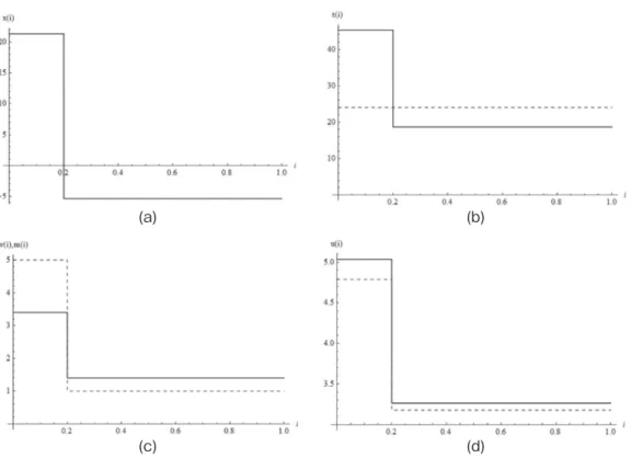
Figure 1 illustrates this case for a given set of parameter values.

(a) (b)

(c) (d)

Figure 1. Case of piecewise linear distribution of initial wealth. (a) Net purchase (positive)

and sale (negative) of time x(i). (b) Pre- and post-trade time under personal control

t(i). (c) Pre-trade money w(i) and post-trade money m(i). (d) Pre- and post-trade

utility. Dashed curves are pre-trade, solid curves are post-trade. Parameter

values used to generate graphs are a=5, b=1, k=0.2, T=24. Each rich agent

consumes 24 + x(0) = 24 + 21.3 = 45.3 hours of human time whereas each poor

agent consumes only 24 + x(1) = 24 – 5.3 = 18.7 hours.

4. Exponential distribution of wealth

To more realistically model the wealth distribution and endogenize the boundary between net buyers and sellers of time, we next examine the case of exponential wealth distribution given by

w(i) = e

, a > 0       (19) Unlike the previous section with two classes each containing many identical agents, agents in this and next sections are all endowed heterogeneously and the division into net sellers and buyers of time arises endogenously as a feature of the equilibrium.

We continue to employ the utility function (10). The necessary condition (5) gives = w(i)−px(i) = p

T＋x(i)

m t        (20)

Solving (20) for x(i) gives

x(i) = w(i)

=

2p T

2 e

2p T

2       (21) The market-clearing condition (1) becomes

−T di = 0

e

p

1

0

       (22) Solving for p yields the market-clearing price:

p = e

aTe

       (23) Equilibrium price (23) is decreasing in a. Since higher values of a correspond to fewer rich and more poor, the equilibrium price is lower when there are fewer rich and more poor agents, as was the case in the two-class economy of the previous section.

The equilibrium distribution of time transactions is 1−e

e

T

x(i) = 2       (24)

To find the borderline agent who is neither a net seller nor a net buyer of time, we solve x(k) = 0 and obtain

log a

e

k = 1− a        (25)

Agents richer than k are net buyers of other agentsʼ time and those poorer are net sellers of their own

time. Moreover, k is decreasing in a, which means that greater wealth inequality corresponds to fewer

buyers of time and more sellers of time.

The distributions of post-trade wealth, time, and utility are, respectively, 1−e

m(i) = 2a        (26)

t(i) =   ＋      T ae

e

T 2        (27)

(ae

(e

4a(e

u(t(i), m(i)) =−a(2i＋1)＋log T          (28)

For every agent, the post-trade utility is weakly greater than pre-trade.

The pre-trade Gini coefficients for the distribution of wealth and time are g

= coth  − ,  g a

= 0,

2 2

a        (29) where coth(z) = e

e

1 2 1

a 1

a 2

g

= g

=  coth 2

      (30) Like in the two-class economy of the previous section, the effect of trade in the exponential case is to reduce wealth inequality by half and generate inequality in time which mirrors the ex-post inequality in wealth.

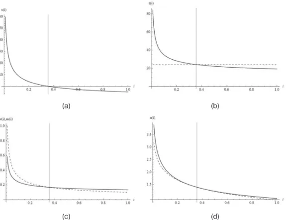
Figure 2 illustrates the case of exponential distribution of wealth for a given set of parameter values.

5. Pareto distribution of wealth

The Pareto distribution better approximates actual wealth and income distributions than the exponential distribution, but is somewhat more difficult to analyze. As a last example, let us consider the Pareto distribution of wealth given by

i

i

a

0 < i

, 1], a∈(0, 1)

w(i) = ,       (31)

Continuing to use the utility function (10) and solving the marginal rate of substitution condition (5) for x(i) gives

2） Unlike the assumption of the unit interval we have used so far, in this section we assume that a unit mass of agents is distributed on [i0, 1].

2p 1 i

i

a

T

x(i) =      − 2       (32)

The market-clearing condition (1) becomes 1 p i

i

a−T di = 0

1 i0

       (33) Solving for p yields the market-clearing price:

(a) (b)

(c) (d)

Figure 2. Case of exponential distribution of initial wealth. (a) Net purchase (positive) and sale (negative) of time x(i). (b) Pre- and post-trade time under personal control t(i).

(c) Pre-trade money w(i) and post-trade money m(i). (d) Pre- and post-trade utility.

Dashed curves are pre-trade, solid curves are post-trade. The vertical line indicates the position of the borderline agent (who is neither a net seller nor a net buyer of time). Parameter values used to generate graphs are a=5 and T=24.

The borderline agent is at 0.32; thus, the wealthiest 32% of agents are net buyers

of time from the 68% of agents who have less wealth. The richest agent

consumes 24 + x(0) = 24 + 48.4 = 72.4 hours of human time whereas the

poorest agent consumes only 24 + x(1) = 24 – 11.6 = 12.4 hours.

i

(1−a)(2＋(1−i

)T)

p =        (34) As in the previous two cases, equilibrium price (34) is decreasing in the parameter of wealth inequality a.

Thus in the Pareto case too, smaller numbers of the rich and greater numbers of the poor lower the equilibrium price of time.

The distribution of time transactions in equilibrium is (1−a)(2＋(1−i

)T)

2(i

) T 2 i

x(i) = i

       (35)

To find the borderline agent who is neither a net seller nor a net buyer of time, we solve x(k) = 0 and obtain

(i

)T (1−a)(2＋(1−i

)T)

−1/a

k = i

       (36)

The borderline agent index k is decreasing in a, which means that greater wealth inequality corresponds to fewer buyers of time and more sellers of time.

The distributions of post-trade wealth and time are, respectively, (i

) (1−a)(2＋(1−i

)T)

1 2 T

i

2 i

m(i) =       ＋

      (37)

i

i (1−a)(2＋(1−i

)T)

2(i

) T 2

t(i) =   −        (38)

As was the case with the exponential distribution, the post-trade utility of each agent u(t(i), m(i)) can be shown to be weakly larger than the pre-trade utility.

The pre-trade Gini coefficients for the distribution of wealth and time are 2−a a

g

=        ,   g

= 0.      (39) The post-trade Gini coefficients are

2−a a i

(2＋(1−i

)T) i

(2＋(2−i

)T)−i

T

g

= g

=        (40) It can be shown that g

> g

∀a ∈ (0, 1), which means trade reduces the inequality in wealth but generates inequality in time which mirrors the ex-post inequality in wealth. To give one numerical example, if a=0.5, i

= 0.01, and T=24, then g

= 0.33 and g

= 0.18. The post-trade wealth inequality is 54% of the pre-trade inequality, not half as in the two previous cases but close.

Figure 3 illustrates the case of Pareto distribution of wealth for a given set of parameter values.

(a) (b)

(c) (d)

Figure 3. Case of Pareto distribution of initial wealth. (a) Net purchase (positive) and sale (negative) of time x(i). (b) Pre- and post-trade time under personal control t(i). (c) Pre-trade money w(i) and post-trade money m(i). (d) Pre- and post-trade utility.

Dashed curves are pre-trade, solid curves are post-trade. The vertical line indicates the position of the borderline agent (who is neither a net seller nor a net buyer of time). Parameter values used to generate graphs are a=0.5, T=24, i

= 0.01. The borderline agent is at 0.36; thus, the wealthiest 35% of agents are net buyers of time from the other 65% of agents who have less wealth. The richest agent consumes 24 + x(0.01) = 24 + 59.6 = 83.6 hours of human time whereas the poorest agent consumes only 24 + x(1) = 24 – 4.8 = 19.2 hours.

6. Extensions

An important extension is to make explicit production and consumption by the agents. The literature

on structural economic dynamics suggests one way to proceed. In particular, Pasinettiʼs (1993) pure-

labor economy is a promising starting point for modeling how agents sell time to produce goods and

then use their earned income to purchase the goods, thereby indirectly paying for the time other agents

spent producing those goods. Since there is no capital in the pure-labor model, the price of each good

corresponds to the cost of the labor required to produce it. What is missing from Pasinettiʼs model is

heterogeneity in wages. Instead of exogenous endowments of wealth, as we have been assuming, agents in the modified Pasinetti framework would be endowed with different wages (due to differences in skills), would earn their income by working, and would spend it on goods that embody the labor time sold by other agents. This formulation would allow identification of net buyers and sellers of time, as well as how wage inequality shapes the pattern of net buying and selling of time in the economy.

Another extension is to broaden the scope to resources besides time which are also endowed equally by nature but reallocated by money, for instance body products (e.g. blood, ova), body organs (e.g.

kidneys), and bodily services (e.g. prostitution, surrogate pregnancy). (Wilkinson 2003, Roth 2015) The broader model would clarify how wealth inequality engenders a reallocation of intrinsic human endowments and thereby compromises the net sellers qua human beings. This extension would complement longstanding efforts on the topic in philosophy, psychology, and sociology by helping operationalize concepts such as dignity and integrity. Particularly pertinent are Kantʼs moral theory, which rejects instrumental use of others and holds price and dignity to be incompatible (Wilkinson 2003, p. 29), and Polanyiʼs economic sociology, which problematizes the “commodity fiction” of labor, land, and money (Polanyi 1944/2001).

A third extension is to find a physical analogue to the way trade readjusts the distribution of the equally-endowed good and the unequally-endowed good. Perhaps the two goods can be represented as two immiscible liquids with different physical properties which are poured one after another into a container of a certain shape. If the way the two liquids settle in the container mirrors the equilibrium of the corresponding economic system, the analogue may lead to new insights and educational applications.

Lastly, the model can be extended to study migration between areas with different distributions of wealth. In particular, a two-country version of the model in which agents first choose whether to migrate and then trade time with compatriots, offers a way to formalize the observations made in the concluding section.

7. Conclusion

Unlike the “work-life balance” perspective, in which quality of life depends on own free time, we conceptualized life satisfaction in terms of the sum of own and othersʼ time at oneʼs disposal. We explicitly modeled time bought and sold, and showed that trade in time reduces wealth inequality but creates inequality in time that mirrors the inequality in wealth.

Our analysis has confirmed what Voltaire famously said back in the 18

century: “The comfort of the rich depends upon an abundant supply of the poor.” We have also confirmed the converse which has gone largely unmentioned: the comfort of the poor depends upon an abundant supply of the rich.

Moreover, we have identified two corollaries: the comfort of the rich [poor] depends on a scarcity of the rich [poor].”

The patterns of migration and political sentiments about it can be interpreted in light of the above

propositions. Poor migrants moving to a country with many rich (or the rural poor moving to the city)

improve not only their own life but also the life of the rich in the new country and the life of the poor in

the old. However, their migration is bad news for the poor in the new country and the rich in the old.

This implies that the poor can be expected to favor policies that restrict immigration but allow emigration, whereas the rich can be expected to favor the opposite.

Another kind of migration involves middle-class residents of rich, low-inequality countries retiring to poor, high-inequality countries. Such migrantsʼ wealth is closer to the rich extreme of the distribution in the new country than in the old. In light of our analysis, such retirees become bigger net buyers of time in the new country than in the old. The local poor welcome them as prospective employers and bidders- up of wages. But their arrival worsens the terms of trade for the local rich vis-à-vis the local poor.

Migration of the moderately well-off from rich egalitarian countries to poor unequal ones, and the pattern of political sentiment concerning such migration, can be understood from the perspective of how such migration affects the terms of trade for time for those who move, for those who stay behind, and for the incumbents in the destination country.

References

Aguiar, Mark and Erik Hurst (2007) “Measuring trends in leisure: the allocation of time over five decades”

Quarterly Journal of Economics 122:3, 969-1006

Barnum, Howard N. and Lyn Squire (1979) “An econometric application of the theory of the farm-household”

Journal of Development Economics 6:1, 79-102

Becker, Gary S. (1965) “A theory of the allocation of time” Economic Journal 75, 493-517 Florida, Richard (2011) The Rise of the Creative Class, Revisited, Basic Books, New York

Gronau, Reuben (1977) “Leisure, Home Production, and Work--the Theory of the Allocation of Time Revisited”

Journal of Political Economy 85:6, 1099-1123

Linder, Staffan B. (1970) The Harried Leisure Class, Columbia University Press, New York

McGrattan, Ellen R. and Richard Rogerson (2004) “Changes in Hours Worked, 1950-2000” Federal Reserve Bank of Minneapolis Quarterly Review 28:1, 14-33

Murray, Charles (2013) Coming Apart: The State of White America, 1960-2010, Crown Publishing, New York Pasinetti, Luigi L. (1993) Structural Economic Dynamics: A Theory of the Economic Consequences of Human

Learning, Cambridge University Press, Cambridge

Polanyi, Karl (1944/2001) The Great Transformation: The Political and Economic Origins of Our Time, Beacon Press, Boston

Roth, Alvin E. (2015) Who Gets What and Why: The New Economics of Matchmaking and Market Design, Houghton Mifflin Harcourt, New York

Temin, Peter (2017) The Vanishing Middle Class: Prejudice and Power in a Dual Economy, MIT Press, Cambridge

Veblen, Thorstein (1899/2007) The Theory of the Leisure Class, Oxford University Press, Oxford

Wilkinson, Stephen (2003) Bodies for Sale: Ethics and Exploitation in the Human Body Trade, Routledge, London