Studies on
Metaheuristics for Continuous Global Optimization Problems
Abdel-Rahman Hedar A. Ahmed
Optimization Problems
Abdel-Rahman Hedar A. Ahmed
Submitted in partial fulfillment of the requirement for the degree of
Doctor of Informatics
Kyoto University Kyoto, Japan
June 2004
Preface
The interface between computer science and operations research has drawn much attention recently especially in optimization which is a main tool in operations research. In optimiza- tion area, the interest on this interface has rapidly increased in the last few years in order to develop nonstandard algorithms that can deal with optimization problems which the stan- dard optimization techniques often fail to deal with. Global optimization problems represent a main category of such problems. Global optimization refers to finding the extreme value of a given nonconvex function in a certain feasible region and such problems are classified in two classes; unconstrained and constrained problems. Solving global optimization prob- lems has made great gain from the interest in the interface between computer science and operations research.
In general, the classical optimization techniques have difficulties in dealing with global optimization problems. One of the main reasons of their failure is that they can easily be entrapped in local minima. Moreover, these techniques cannot generate or even use the global information needed to find the global minimum for a function with multiple local minima.
The interaction between computer science and optimization has yielded new practical solvers for global optimization problems, calledmetaheuristics. The structures of metaheuristics are mainly based on simulating nature and artificial intelligence tools. Metaheuristics mainly invoke exploration and exploitation search procedures in order to diversify the search all over the search space and intensify the search in some promising areas. Therefore, metaheuristics cannot easily be entrapped in local minima. However, metaheuristics are computationally costly due to their slow convergence. One of the main reasons for their slow convergence is that they may fail to detect promising search directions especially in the vicinity of local minima due to their random constructions.
In this study, both global optimization problem classes; unconstrained and constrained problems, are considered in the continuous search space. New hybrid versions of metaheuris- tics are proposed as promising solvers for the considered problems. The proposed methods
aim to overcome the drawbacks of slow convergence and random constructions of meta- heuristics. In these hybrid methods, local search strategies are inlaid inside metaheuristics in order to guide them especially in the vicinity of local minima, and overcome their slow convergence especially in the final stage of the search.
Metaheuristics are derivative-free methods so that direct search methods, which are also derivative-free methods, are invoked to play the role of local search in the proposed hybrid methods. Therefore, the hybrid methods proposed in this study confront the growth of many optimization problems in which the gradient information is not available.
Kyoto, Japan Abdel-Rahman Hedar A. Ahmed
June 2004
Acknowledgements
I am greatly indebted to my supervisor, Prof. Masao Fukushima, one of the great scientists in optimization and mathematical programming, for many things. I thank him for accepting me to be one of his students in Kyoto University from four years ago, for his suggestion of this research area to work on, and for his direct supervision. I would also like to thank him for his continual suggestions and support during this research. I owe special thanks for him for carefully reading and invaluable suggestions and corrections of the draft manuscripts of the parts of this thesis.
I would like to thank all members of Prof. Fukushima’s research group, Prof. Tetsuya Takine, Dr. Nobuo Yamashita and my colleagues, for the good scientific atmosphere they offered to me during my study in Kyoto University. I would also like to thank Prof. Toshihide Ibaraki and Dr. Mutsunori Yagiura for providing me with some essential research papers needed in my study from their own libraries. Moreover, I am very grateful that I have been graduated from Kyoto University, one of the best universities in Japan and all over the world.
I owe thanks to Egyptian Government and Kyoto University for supporting my study in Japan. I am grateful for all research facilities that have been provided to me in Kyoto University to achieve this study.
Although I was very happy to be a great scientific environment represented in Kyoto University, it was hard to achieve the needed research atmosphere without my wife’s support.
Actually, it was not so easy for me to be settled in an oriental culture like Japanese Culture without her accompany. So, I am very grateful for her continual supports and encouragement.
I owe great thanks to my great parents for all things that they gave to me or taught me.
Without their supports I would never have made any success.
I have been brought up in an Islamic culture and environment in which my parents taught me importance of thanks and appreciation to others and primarily to Allah, the Creator, the Ultimate Source of all gifts in life. I have been always grateful to their teaching so lastly
and above all, I would thank Him Almighty for all His gifts, guidance and helps.
Contents
Preface i
Acknowledgements iii
1 Introduction 1
1.1 Continuous Global Optimization Problems . . . 2
1.2 Metaheuristics . . . 3
1.2.1 Genetic Algorithms . . . 3
1.2.2 Simulated Annealing . . . 6
1.2.3 Tabu Search . . . 8
1.3 Direct search methods . . . 9
1.3.1 Nelder-Mead method . . . 10
1.3.2 Pattern Search methods . . . 13
1.4 Organization and Contributions . . . 14
2 Direct Search SA for Unconstrained Global Optimization 17 2.1 Introduction . . . 17
2.2 The description of the proposed methods . . . 18
2.2.1 Simple direct search (SDS) . . . 19
2.2.2 Simplex simulated annealing (SSA) . . . 21
2.2.3 Direct search simulated annealing (DSSA) . . . 22
2.3 Experimental results . . . 24
2.3.1 Setting of parameters . . . 25
2.3.2 Numerical results . . . 26
2.4 Conclusion . . . 29
3 Simplex Coding GA for Unconstrained Global Optimization 33 3.1 Introduction . . . 33
3.2 Simplex-Based Genetic Algorithms . . . 34
3.3 Description of SCGA . . . 36
3.3.1 Initialization . . . 36
3.3.2 GA loop . . . 37
3.3.3 Acceleration in the final stage . . . 39
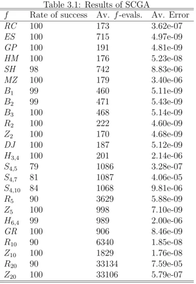
3.4 Experimental Results . . . 40
3.4.1 Parameter setting . . . 40
3.4.2 Numerical results . . . 42
3.5 Conclusion . . . 46
4 Heuristic Pattern Search SA for Unconstrained Global Optimization 47 4.1 Introduction . . . 47
4.2 Approximate Descent Direction . . . 48
4.3 Heuristic Pattern Search . . . 54
4.4 Simulated Annealing HPS . . . 59
4.5 Experimental Results . . . 62
4.5.1 Setting of Parameters . . . 62
4.5.2 Numerical Results . . . 63
4.6 Conclusion . . . 65
5 Directed TS for Unconstrained Global Optimization 67 5.1 Introduction . . . 67
5.2 TS Memory Elements . . . 69
5.2.1 Multi-Ranked Tabu List (TL) . . . 70
5.2.2 Visited Region List (VRL) . . . 72
5.3 Neighborhood-Local Search Strategies . . . 73
CONTENTS vii
5.3.1 Nelder-Mead Search (NMS) Strategy . . . 74
5.3.2 Adaptive Pattern Search (APS) Strategy . . . 74
5.4 Directed Tabu Search (DTS) . . . 76
5.4.1 Exploration-Diversification Loop . . . 77
5.4.2 Intensification Search . . . 79
5.4.3 Main Algorithm . . . 79
5.5 Implementation and Experiments . . . 82
5.5.1 Setting Parameters . . . 82
5.5.2 Numerical Results . . . 85
5.6 Conclusion . . . 92
6 Filter SA for Constrained Global Optimization 93 6.1 Introduction . . . 93
6.2 Preliminaries . . . 95
6.2.1 Pareto Dominance . . . 96
6.2.2 Problem Reformulation . . . 96
6.2.3 Filter Set and Filtered Points . . . 97
6.3 The FSA method . . . 97
6.3.1 Diversification Generation Procedure . . . 98
6.3.2 Ranking Procedure . . . 100
6.3.3 Trial Solution Generation Procedure . . . 101
6.3.4 Intensification . . . 102
6.3.5 FSA Algorithm . . . 103
6.4 Setting FSA Parameters . . . 104
6.4.1 Constraint Violation Function Parameters . . . 105
6.4.2 Diversification Parameters . . . 106
6.4.3 Cooling Schedule Parameters . . . 106
6.4.4 Trial Solutions Parameters . . . 106
6.4.5 Intensification Parameters . . . 107
6.5 Numerical Results . . . 107
6.6 More Numerical Experiments . . . 110
6.6.1 Welded Beam Design Problem . . . 110
6.6.2 Pressure Vessel Design Problem . . . 113
6.6.3 Tension-Compression String Problem . . . 113
6.7 Conclusion . . . 114
7 Summary and Conclusions 115
A Unconstrained Test Problems 117
B Constrained Test Problems 125
Chapter 1 Introduction
Many recent problems in science, engineering and economics can be expressed as comput- ing globally optimal solutions [48, 49, 74, 75, 76]. Using classical nonlinear programming techniques may fail to solve such problems because these problems usually contain multiple local optima. Therefore, global search methods should be invoked in order to deal with such problems. In recent years, there has been a great deal of interest in emerging some artificial intelligence tools in the area of optimization. These tools which are normally called metaheuristics are mainly proposed by simulating nature or by invoking intelligent learned procedures [30, 73, 81].
One main category of global optimization problems contains the problems which are characterized by one or more of the following properties:
• Calculation of the objective function (or constraint functions if exist) is very expensive or time consuming.
• The exact gradient of the objective function (or constraint functions if exist) cannot be computed, or its numerical approximation is very expensive or time consuming.
• The values of the objective function (or constraint functions if exist) contain noise.
Such problems exist in many real-world applications and achieving the exact global solution is neither possible nor desirable. Therefore, using derivative-free global search methods is highly needed in order to achieve acceptable solutions. Actually, metaheuristics fight courageously when applied to these problems and they could obtain highly accurate solutions in many cases [73]. The power of metaheuristics comes from the fact that they are robust and can deal successfully with a wide range of problem areas. However, these methods, especially when they are applied to complex problems, suffer from the slow convergence that
brings about the high computational cost. The main reason for this slow convergence is that these methods explore the global search space by creating random movements without using much local information about promising search direction. In contrast, local search methods have faster convergence due to their using local information to determine the most promising search direction by creating logical movements. However, local search methods can easily be entrapped in local minima.
One approach that recently has drawn much attention is to combine metaheuristics with local search methods to design more efficient methods with relatively faster convergence than the pure metaheuristics, see [37, 38, 39, 40, 41, 42] and references therein. Moreover, these hybrid methods are not easily entrapped in local minima because they still maintain the merits of the metaheuristics.
In this study, new hybrid methods that combine metaheuristics and direct search meth- ods are proposed in order to deal with the global optimization problems that have the above characteristics. Specifically, local search guidance in the direct search methods is invoked to direct and control the global search features of metaheuristics to design more efficient hybrid methods. In the rest of this chapter, some well-known direct search methods and metaheuris- tics are introduced to be used throughout this study. The mathematical definitions of the considered problems are given first.
1.1 Continuous Global Optimization Problems
In this study, both unconstrained and constrained global optimization problems in a continu- ous space are considered. Without loss of generality, only minimization problems are studied since maximization problems can be transformed to minimization problems by inverting the sign of their objective functions. The mathematical definitions for the considered problems are given below.
Unconstrained Problem
minxǫRn f(x), (1.1.1)
wheref is a generally nonconvex, real valued function defined onRn. Constrained Problem
minx f(x),
s.t. gi(x)≤0, i= 1, . . . , l, hj(x) = 0, j = 1, . . . , m, x∈ S,
(1.1.2)
1.2 Metaheuristics 3
where f , gi and hj are real-valued functions defined on the search space S ⊆Rn. Usually, the search space S is defined as {x∈Rn:xi ∈[li, ui], i= 1, . . . , n}.
1.2 Metaheuristics
The term “metaheuristics” was first proposed by Glover [27]. The word “metaheuristics”
contains all heuristics methods that show evidence of achieving good quality solutions for the problem of interest within an acceptable time. Usually, metaheuristics offer no guarantee of obtaining the global solutions.
Metaheuristics can be classified into two classes; population-based methods and point- to-point methods. In the latter methods, the search invokes only one solution at the end of each iteration from which the search will start in the next iteration. On the other hand, the population-based methods invoke a set of many solutions at the end of each iteration.
Below, we highlight the principles of genetic algorithm as an example of population-based methods, and simulated annealing and tabu search as examples of point-to-point methods.
1.2.1 Genetic Algorithms
A genetic algorithm (GA) is a procedure that tries to mimic the genetic evolution of a species.
Specifically, GA simulates the biological processes that allow the consecutive generations in a population to adapt to their environment. The adaptation process is mainly applied through genetic inheritance from parents to children and through survival of the fittest. Therefore, GA is a population-based search methodology. Some pioneering works traced back to the middle of 1960s preceded the main presentation of the GAs of Holland [46] in 1975. However, GAs were limitedly applied until their multipurpose presentation of Goldberg [34] in search, optimization, design and machine learning areas. Nowadays, GAs are considered to be the most widely known and applicable type of metaheuristics [7, 8, 68].
GA starts with an initial population whose elements are called chromosomes. The chro- mosome consists of a fixed number of variables which are called genes. In order to evaluates and rank chromosomes in a population, a fitness function based on the objective function should be defined. Three operators must be specified to construct the complete structure of the GA procedure; selection, crossover and mutation operators. The selection operator cares with selecting an intermediate population from the current one in order to be used by the other operators; crossover and mutation. In this selection process, chromosomes with
higher fitness function values have a greater chance to be chosen than those with lower fitness function values. Pairs of parents in the intermediate population of the current generation are probabilistically chosen to be mated in order to reproduce the offspring. In order to in- crease the variability structure, the mutation operator is applied to alter one or more genes of a probabilistically chosen chromosome. Finally, another type of selection mechanism is applied to copy the survival members from the current generation to the next one.
GA operators; selection, crossover and mutation have been extensively studied. Many effective setting of these operators have been proposed to fit a wide variety of problems. More details about GA elements are discussed below before stating a standard GA in Algorithm 1.2.1.
Fitness Function
Fitness functionF is a designed function that measures the goodness of a solution. It should be designed in the way that better solutions will have a higher fitness function value than worse solutions. The fitness function plays a major role in the selection process.
Coding
Coding in GA is the form in which chromosomes and genes are expressed. There are mainly two types of coding; binary and real. The binary coding was presented in the GA original presentation [46] in which the chromosome is expressed as a binary string. Therefore, the search space of the considered problem is mapped into a space of binary strings through a coder mapping. Then, after reproducing an offspring, a decoder mapping is applied to bring them back to their real form in order to compute their fitness function values. Actually, many researchers still believe that the binary coding is the ideal. However, the real coding is more applicable and easy in programming. Moreover, it seems that the real coding fits the continuous optimization problems better than the binary coding [44].
Selection
Consider a population P, selection operator selects a set P′ ⊆ P of the chromosomes that will be given the chance to be mated and mutated. The size of P′ is the same as that of P but more fit chromosomes in P are chosen with higher probability to be included in P′. Therefore, the most fit chromosomes inP may be represented by more than one copy in P′ and the least fit chromosomes inP may be not represented at all inP′.
1.2 Metaheuristics 5
Consider the populationP ={x1, x2, . . . , xN}. The difference between selection operators lies in the way of computing the probability of including a copy of chromosomexi ∈P into the setP′, which is denoted by ps(xi). Using these probabilities, the population is mapped onto a roulette wheel, where each chromosome xi is represented by a space that proportionally corresponds to ps(xi). Chromosomes in the set P′ are chosen by repeatedly spinning the roulette wheel until all positions in P′ are filled.
The most common selection operators are theproportional selection [46] andlinear rank- ing selection [9], see [6] for ease of explanation and comparison of different selection op- erators. It is noteworthy that in the proportional selection mechanism, the probabilities ps(xi), i= 1, . . . , N, are calculated by
ps(xi) = F(xi) PN
j=1F(xj).
whereF is the fitness function which must have positive values for all possible chromosomes in order to be used in this selection mechanism. In linear ranking selection mechanism, the chromosomes of P are sorted in the order of raw fitness, i.e.,
F(x1)≤F(x2)≤ · · · ≤F(xN).
Then the probabilities ps(xi), i= 1, . . . , N, are calculated by ps(xi) = 1
M µ
ηmax−(ηmax−ηmin) i−1 N −1
¶ , where ηmin = 2−ηmax and 1≤ηmax ≤2.
Crossover and Mutation
Crossover operator aims to interchange the information and genes between chromosomes.
Therefore, crossover operator combines two or more parents to reproduce new children, then, one of these children may hopefully collect all good features that exist in his parents.
Crossover operator is not typically applied for all parents but it is applied with probability pc which is normally set equal to 0.6. Actually, crossover operator plays a major role in GA, so defining a proper crossover operator is highly needed in order to achieve a better performance of GA. Different types of crossover operators have been studied, see [44] as a condensed survey.
Mutation operator alters one or more gene in a chromosome. Mutation operator aims to achieve some stochastic variability of GA in order to get a quicker convergence. The probability pm of applying the mutation operator is usually set to be small, normally 0.01.
Algorithm 1.2.1. Genetic Algorithm
1. Initialization. Generate an initial population P0. Set the crossover and mutation probabilities pc ∈(0,1) and pm ∈(0,1), respectively. Set the gener- ation counter t:= 1.
2. Selection. Evaluate the fitness function F at all chromosomes in Pt. Select an intermediate population Pt′ from the current population Pt.
3. Crossover. Associate a random number from (0,1) with each chromosome in Pt′ and add this chromosome to the parents pool set StP if the associated number is less than pc. Repeat the following Steps 3.1 and 3.2 until all parents in StP are mated:
3.1. Choose two parents p1 and p2 from StP. Mate p1 and p2 to reproduce children c1 and c2.
3.2. Update the children pool set StC throughStC :=StC ∪ {c1, c2} and update StP through StP :=StP − {p1, p2}.
4. Mutation. Associate a random number from (0,1) with each gene in each chromosome in Pt′, mutate this gene if the associated number is less than pm, and add the mutated chromosome only to the children pool set StC.
5. Stopping Conditions. If stopping conditions are satisfied, then terminate.
Otherwise, select the next generation Pt+1 from Pt∪StC. Set StC to be empty, set t:=t+ 1, and go to Step 2.
1.2.2 Simulated Annealing
The original ideas of the simulated annealing (SA) methods dates back to 50s of the last cen- tury. Exactly, in 1953, Metropolis et al. [65] introduced an efficient algorithm to simulated the equilibrium of a collection of atoms at a given temperature. This pioneering technique
1.2 Metaheuristics 7
had inspired Kirkpatrik et al. [53] to simulate it in optimization and call it Simulated An- nealing (SA). Since the presentation of Kirkpatrik et al., a lot of studies that invoke SA have emerged in the area of optimization. Actually, the theoretical aspects as well as the applications of SA have been extensively studied, see [58, 57] and see [1, 43] as recent and short surveys.
The SA algorithm successively generates a trial point in a neighborhood of the current solution and determines whether or not the current solution is replaced by the trial point based on a probability depending on the difference between their function values. Conver- gence to an optimal solution can theoretically be guaranteed only after an infinite number of iterations controlled by the procedure so-called cooling schedule. The main control pa- rameter in the cooling schedule is the temperature parameter T. The main role of T is to let the probability of accepting a new move be close to 1 in the earlier stage of the search and to let it be almost zero in the final stage of the search. A proper cooling schedule is needed in the finite-time implementation of SA to simulate the asymptotic convergence behavior of the SA. Algorithm 1.2.2 states the steps of the standard SA method.
Algorithm 1.2.2. Simulated Annealing
1. Initialization. Choose an initial solution x0, and fix the cooling schedule parameters; initial temperature Tmax, epoch length M, cooling reduction ratio λ ∈ (0,1), and minimum temperature Tmin. Set the temperature T := Tmax and k := 0.
2. Epoch Loop. Repeat the following steps (2.1–2.3) M times.
2.1. Generate a trial point yk in the neighborhood of the current solution xk. 2.2. Evaluate f on the trial point yk, and compute
p:=
1, if f(yk)< f(xk);
exp¡−∆f
T
¢, otherwise,
where ∆f :=f(yk)−f(xk).
2.3. Choose a random numberufrom(0,1).Ifp≥u, setxk+1 :=yk. Otherwise, set xk+1 :=xk. Set k :=k+ 1.
3. Termination Condition. If the cooling schedule is completed (T ≤Tmin), terminate. Otherwise, decrease the temperature by setting T := λT, and go to Step 2.
One of the most powerful features of SA is its ability of easily escaping from being trapped in local minima by accepting up-hill moves through a probabilistic procedure especially in the earlier stages of the search. On the other hand, the main drawbacks that have been noticed on SA are its suffering from slow convergence and its wandering around the optimal solution if high accuracy is needed.
1.2.3 Tabu Search
Tabu Search (TS) is a heuristic method originally proposed by Glover in 1986 [27]. TS has been proposed and developed for combinatorial optimization problems [28, 29, 31]. TS fights courageously when applied to combinatorial optimization problems [31, 73, 81]. However, there is a very limit number of TS contributions in continuous optimization problems [39].
The main feature of TS is its use of an adaptive memory and responsive exploration.
A simple TS combines a local search procedure with anti-cycling memory-based rules to prevent the search from getting trapped in local minima. Specifically, TS restricts returning to recently visited solutions by constructing a list of them called Tabu List (TL). In each iteration of the simple TS illustrated in Algorithm 1.2.3, TS generates many trial solutions in a neighborhood of the current solution. The trial solutions generation process is composed to avoid generating any trial solution that is already recently visited. The best trial solution found among the generated solutions will become the next solution. Therefore, TS can accept uphill movements to avoid getting trapped in local minima. TS can be terminated if the number of iterations without any improvement exceeds a predetermined maximum number.
Algorithm 1.2.3. Simple Tabu Search
1. Choose an initial solution x0. Set the Tabu List (TL) to be empty, and set the counter k:= 0.
2. Generate neighborhood moves list M(xk) = {x′ :x′ ∈ N(xk)}, based on tabu restrictions, where N(xk) is a neighborhood of xk.
1.3 Direct search methods 9
3. Set xk+1 equal to the best trial solution in M(xk), and update TL.
4. If stopping conditions are satisfied, terminate. Otherwise, go to Step 2.
A simple TS structure given in Algorithm 1.2.3 is calledshort-term memory TS. Updating the memory-based TL can be modified and controlled by the following concepts:
• Tabu tenure: number of iterations in which a tabu move is considered to remain tabu or forbidden;
• Aspiration criteria: accepting an improving solution even if generated by a tabu move.
The short-term memory is built to keep the recency only. In order to achieve better per- formance, long-term memory has been proposed to keep more important search features besides the recency, such as the quality and the frequency [32]. Specifically, long-term mem- ory in high-level TS records attributes of special characters like elite and frequently visited solutions. Then, the search process of TS can adapt itself by using these special types of solutions in:
• Intensification: giving priority to elite solutions in order to obtain much better solutions in their vicinity.
• Diversification: discouraging attributes of frequently visited solutions in new move selection functions in order to diversify the search to other areas of solution space.
1.3 Direct search methods
Direct search methods can be simply defined as the procedures which try to direct the search for a minimum through the geometric intuition of the objective function by using function values only without evaluating the gradients, see [54, 78, 93]. In order to show the reality and the difficulty of the job that has been delegated to direct search methods, we borrow John Dennis’ description of these methods which is stated and extended by Mike Powell in [77]:
“It is to find the deepest point of a muddy lake, given a boat and a plump line, when there is a price to be paid for each sounding. A specification of an algorithm that is suitable for solving this problem would probably appeal to
geometric intuition, and probably the procedure would require widely spaced measurements to be taken, in order to smooth out any high frequency variations in the depth of the lake. Experience has shown that many computer users find such algorithms attractive for a wide range of optimization calculations.”
Direct search methods were originally proposed in the 1950s and 1960s to be justified in terms of geometric intuition in low dimensional spaces without mathematical proof. Since these methods are simple, easy to understand, easy to program, and widely applicable, they have remained popular for real-world problems in chemistry, chemical engineering and medicine. However, they failed to attract the mathematical optimization community until the appearance of their mathematical analysis from only fifteen years ago. In this section, Nelder-Mead and pattern search methods are presented as examples of direction search methods.
1.3.1 Nelder-Mead method
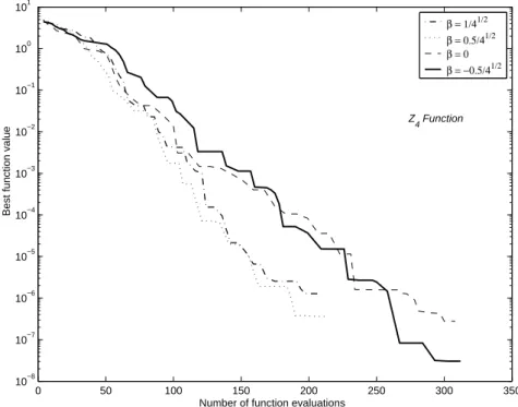
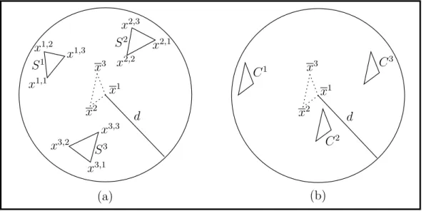
The local search method called the Nelder-Mead method [72] is one of the most popular derivative-free nonlinear optimization methods. Instead of using the derivative information on the function to be minimized, the Nelder-Mead method maintains at each iteration a nondegenerate simplex, a geometric figure in n dimensions of nonzero volume that is the convex hull of n+ 1 vertices, x1, x2, . . . , xn+1, and their respective function values. In each iteration, new points are computed, along with their function values, to form a new simplex.
Four scalar parameters must be specified to define a complete Nelder-Mead method; coef- ficients of reflection ρ, expansion χ, contraction γ, and shrinkage σ. These parameters are chosen to satisfy
ρ >0, χ >1, 0< γ < 1, and 0< σ <1.
The Nelder-Mead method consists of the following steps:
Algorithm 1.3.1. Nelder-Mead Method
1. Order. Order and re-label the n + 1 vertices as x1, x2, . . . , xn+1 so that f(x1)≤f(x2)≤ · · · ≤f(xn+1). Since we want to minimizef, we refer tox1
as the best vertex or point, to xn+1 as the worst point.
1.3 Direct search methods 11
2. Reflect. Compute the reflection point xr by xr =x+ρ(x−xn+1),
where x is the centroid of the n best points, i.e., x = Pn
i=1xi/n. Evaluate f(xr). If f(x1)≤f(xr)< f(xn), replace xn+1 with the reflected point xr and go to Step 6.
3. Expand. If f(xr)< f(x1), compute the expansion point xe by xe =x+χ(xr−x).
Evaluate f(xe). If f(xe) < f(xr), replace xn+1 with xe and go to Step 6;
otherwise replace xn+1 with xr and go to Step 6.
4. Contract. If f(xr)≥f(xn), perform a contraction between xand the better of xn+1 and xr.
4.1. Outside. If f(xn) ≤ f(xr) < f(xn+1) (i.e., xr is strictly better than xn+1), perform an outside contraction: Calculate
xoc=x+γ(xr−x).
Evaluate f(xoc). If f(xoc) ≤ f(xr), replace xn+1 with xoc and go to Step 6;
otherwise, go to Step 5.
4.2. Inside. Iff(xr)≥f(xn+1), perform an inside contraction: Calculate xic=x+γ(xn+1−x).
Evaluate f(xic). If f(xic)≤ f(xn+1), replace xn+1 with xic and go to Step 6;
otherwise, go to Step 5.
5. Shrink. Evaluate f at the n new vertices
x′i =x1 +σ(xi−x1), i= 2, . . . , n+ 1.
x1
x3
x2 x2
x1
x3
xic
xoc xr
xe
x′3
x′2
Figure 1.1: The reflection, expansion, contraction and shrinkage points for a simplex in two dimensions.
Replace the vertices x2, . . . , xn+1with the new vertices x′2, . . . , x′n+1.
6. Stopping Condition. Order and re-label the vertices of the new simplex as x1, x2, . . . , xn+1 such that f(x1) ≤ f(x2) ≤ · · · ≤ f(xn+1). If f(xn+1)− f(x1)< ε, then stop, whereε >0 is a small predetermined tolerance. Other- wise, go to Step 2.
Figure 1.1 shows the effects of reflection, expansion, contraction and shrinkage for a simplex in two dimensions using the standard values of the coefficients
ρ= 1, χ= 2, γ = 1
2, and σ = 1 2.
After more than thirty years of studying and applying the Nelder-Mead method, McKin- non [64] shows that the Nelder-Mead algorithm can stagnate and converge to a nonoptimal point even for very simple problems. However, Kelley [51, 52] proposes a test for sufficient decrease which, if passed for all iterations, will guarantee convergence of the Nelder-Mead iteration to a stationary point under some appropriate conditions. Moreover, he modified the Nelder-Mead method by invoking a reconstruction of the simplex called “oriented restarts” whenever the decrease test does not hold. This new orientation of the simplex is intended to
1.3 Direct search methods 13
compensate for the kind of stagnation that was exhibited in [64]. However, this modification improves the robustness of the method, but it does not solve all the problems on stagnation of the Nelder-Mead method.
1.3.2 Pattern Search methods
Pattern search methods direct the search towards a local minimum through a pattern con- taining a certain number of points. Although the original pattern search algorithm has been proposed by Hooke and Jeeves [47], the pattern search methods as well as other direct search methods were not wildly applicable until fifteen years ago. The renaissance of pattern search methods began in 1989 with Torczon’s Ph. D. thesis [87] and reached its mature stage by her paper [88] in which she has presented the generalized pattern search (GPS) as a framework of pattern search methods.
Pattern search methods invoke a pattern containing at leastn+1 points in each iteration.
One of these points is the current iterate and the other point are generated along search directions starting from the current iterate with a certain step size. The search directions used to generate the pattern points consist of a finite set of positive spanning directions in Rn. However, in order to achieve quicker convergence, other promising search directions may be included in addition to the positive spanning directions. Whenever the search fails to obtain a better movement, the step size is decreased in order to refine the search.
A sample GPS algorithm is stated in Algorithm 1.3.2 based on the one presented in [4].
In the initialization step of GPS, a set D of positive spanning directions in Rn should be chosen beside the initial solution and step size. For example, the set D can be set either {e1, . . . , en,−e1, . . . ,−en}or{e1, . . . , en,−e},whereei ∈Rnis theith unit vector inRnand e ∈Rn is the vector of ones. In each iteration of GPS, the mesh point set Mk and the poll points set Pk based on the set D should be computed as
Mk ={y:y=xk+ ∆kdz ∈X, d∈D, z ∈Z+|D|}, (1.3.1) Pk={y:y=xk+ ∆kd ∈X, d∈Dk}, (1.3.2) where Z+ is the set of all positive integers. Moreover, the step size ∆k is updated at each iteration in the way that it remains the same as its previous setting, or it is increased whenever an improvement is achieved, and it is decreased otherwise. More details about the step size updating process is given in [88] in order to fulfill some assumptions needed in the mathematical analysis of GPS.
The scenario of GPS starts with fitting the initial parameters, and then two search stages are invoked before the updating step. The first search stage is called Search Step in which any search procedure can be defined by the user to generate trial solutions from Mk. The main role of theSearch Step is to achieve faster convergence of GPS. The other search stage called Poll Step is invoked as a systematic search in order to explore a region around the current solution. If an improvement is obtained, then the search is going on with the same step size or with a bigger step size if more promising solutions are expected. Otherwise, the current iterate is called a mesh optimizer and the step size is reduced in order to refine the mesh. GPS may be terminated when the step size becomes small enough.
Algorithm 1.3.2. Generalized Pattern Search
1. Initialization. Choose an initial solution x0, choose a positive spanning directions set D, choose a step size ∆0 > 0 and set the counter number k := 0.
2. Search Step: Compute the meshMk as in (1.3.1). Invoke a search strategy to get an improved point from Mk. If an improvement is obtained go to Step 4.
3. Poll Step. Choose the search direction set Dk ⊂D to be used in computing the poll set Pk as in (1.3.2). Evaluate f at all points in Pk.
4. Update Step. If an improved point obtained in Step 2 or 3, set xk+1 equal to this improved point, and set ∆k+1 ≥ ∆k. Otherwise, set xk+1 := xk, and
∆k+1 <∆k.
5. Termination Conditions. If the termination conditions are satisfied, then stop. Otherwise, set k:=k+ 1, and go to Step 2.
1.4 Organization and Contributions
In the subsequent chapters, we will introduce new hybrid methods that deal with the con- tinuous global optimization problems in their two forms; unconstrained and constrained
1.4 Organization and Contributions 15
problems. Below, we summarize the organization of the rest of the thesis as well as brief descriptions of the main contributions done in this study.
In Chapter 2, we give a new approach of hybrid direct search methods with metaheuristics of simulated annealing for finding a global minimum of a nonlinear function with continuous variables. First, we suggest a Simple Direct Search (SDS) method, which comes from some ideas of other well known direct search methods. Since our goal is to find global minima and the SDS method is still a local search method, we hybridize it with the standard simulated annealing to design a new method, called Simplex Simulated Annealing (SSA) method, which is expected to have some ability to look for a global minimum. To obtain faster convergence, we first accelerate the cooling schedule in SSA, and in the final stage, we apply Kelley’s modification of the Nelder-Mead method on the best solutions found by the accelerated SSA method to improve the final results. We refer to this last method as the Direct Search Simulated Annealing (DSSA) method. The performance of SSA and DSSA is reported through extensive numerical experiments on some well known functions.
In Chapter 3, a new algorithm called Simplex Coding Genetic Algorithm (SCGA) is proposed by hybridizing genetic algorithm and Nelder-Mead method. In the SCGA, each chromosome in the population is a simplex and the gene is a vertex of this simplex. Selection, new multi-parents crossover and mutation procedures are used to improve the initial pop- ulation. Moreover, Nelder-Mead method is applied to improve the population in the initial stage and every intermediate stage when new children are generated. Applying Nelder- Mead method again on the best point visited is the final stage in the SCGA to accelerate the search and to improve this best point. The efficiency of SCGA is tested on some well known functions.
In Chapter 4, we present a new approach of hybrid simulated annealing method for minimizing multimodel functions called the simulated annealing heuristic pattern search (SAHPS) method. Two subsidiary methods are proposed to achieve the final form of the global search method SAHPS. First, we introduce the approximate descent direction (ADD) method, which is a derivative-free procedure with high ability of producing a descent di- rection. Then, the ADD method is combined with a pattern search method with direction pruning to construct the heuristic pattern search (HPS) method. The last method is hy- bridized with simulated annealing to obtain the SAHPS method. The experimental results through well-known test functions are shown to demonstrate the efficiency of the SAHPS method.
In Chapter 5, we introduce a continuous TS called Directed Tabu Search (DTS) method.
In the DTS method, direct-search-based strategies are used to direct a tabu search. These
strategies are based on the well-known Nelder-Mead method and a new pattern search proce- dure called adaptive pattern search. Moreover, we introduce a new tabu list conception with anti-cycling rules called Tabu Regions and Semi-Tabu Regions. In addition, Diversification and Intensification search schemes are employed. Numerical results of the DTS method are reported through extensive numerical experiments on several well known functions.
In Chapter 6, a simulated-annealing-based method called Filter Simulated Annealing (FSA) method is proposed to deal with the constrained global optimization problem. The considered problem is reformulated so as to take the form of optimizing two functions; the objective function and the constraint violation function. Then, the FSA method is applied to solve the reformulated problem. The FSA method invokes a multi-start diversification scheme in order to achieve an efficient exploration process. To deal with the considered problem, a filter-set-based procedure is built in the FSA structure. Finally, an intensification scheme is applied as a final stage of the proposed method in order to overcome the slow convergence of SA-based methods. The computational results obtained by the FSA method are reported and compared with some population-based methods.
Chapter 7 gives brief summary and conclusions of the main contributions in the thesis.
Finally, the unconstrained test problems and the constrained test problems used throughout the study are given in Appendixes A and B, respectively.
Chapter 2
Direct Search SA for Unconstrained Global Optimization
2.1 Introduction
One approach that recently has drawn much attention is to combine simulated annealing (SA) method with local search methods to design more efficient methods with relatively faster convergence than the pure SA methods. Direct search methods, as local search methods, have got much attention in these combinations. For instance, SA was hybridized with simplex- based direct search method in [13, 79]. In addition, Kvasnicka and Pospichal [56] proposed a hybrid of controlled random search method, which is a generalization of the Nelder-Mead method, and SA.
In this chapter, we will hybridize SA and direct search methods to deal with the uncon- strained optimization problem
minxǫRn f(x), (2.1.1)
where f is a generally nonconvex, real valued function defined on Rn. First, we suggest a simple direct search (SDS) method, which comes from some ideas of other well known direct search methods. Since our goal is to find global minima and the SDS method is still a local search method, we hybridize it with the standard simulated annealing to design a new method, called simplex simulated annealing (SSA) method, which is expected to have some ability to look for global minima. The final method, called the direct search simulated annealing (DSSA) method, can be obtained by modifying SSA. To obtain faster convergence, we first accelerate the cooling schedule in SSA, and in the final stage, we apply Kelley’s modification of the Nelder-Mead method [51, 52] on the best solutions found by the accelerated SSA to improve the final results. These two modifications on SSA will comprise
the final method DSSA. The performance of SSA and DSSA is reported through extensive numerical experiments on some well known functions. Comparing their performance with that of other metaheuristics methods shows that SSA and DSSA are promising in practice.
Especially, DSSA is shown to be very efficient and robust.
To the author’s knowledge, there are two main previous results on hybridizing simulated annealing with simplex methods. Press and Teukolsky [79] add a positive logarithmically distributed variable, proportional to the control annealing temperature T, to the function associated with every vertex of the simplex. Likewise, they subtract a similar random variable from the function value at every new replacement point. Then, their method may accept a new simplex whose actual function values at its vertices are not better than those at the previous simplex. This method was subsequently studied by Cardoso et al. [13, 14]. The other main result was presented by Kvasnicka and Pospichal [56]. Their method depends on the use of the simulated annealing acceptance in a controlled random search method. More precisely, the controlled random search uses a simplex method on randomly selected simplex sets from the population. So, to avoid being entrapped in local minima, they applied simulated annealing acceptance on the updating procedure. The common idea underlying these hybrid approaches and also our approach is to use simplex method to generate new logical movements while applying simulated annealing. However, the approach proposed in this chapter is different from the above mentioned approaches. We try to fix some disadvantages of simulated annealing like its slowness and its wandering near the global minimum in the final stage of search. So, we use a new simplex method to generate the movements trying to explore the function domain more carefully while applying accelerated simulated annealing, and also use another simplex method to accelerate the final stage in the search.
This chapter is organized as follows. In Section 2.2, we state the description of the proposed methods. Experimental results along with the initialization of some parameters and the setting of the control parameters of the proposed methods are discussed in Section 2.3. The conclusion of the contribution of this chapter makes up Section 2.4.
2.2 The description of the proposed methods
In this section, we describe the SDS, SSA and DSSA methods and introduce the initial and control parameters that are required by these methods. The values of these parameters used in the experiments will be given in Section 2.3.
2.2 The description of the proposed methods 19
2.2.1 Simple direct search (SDS)
Before we state the steps of the SDS method, we will introduce the main ideas which SDS comes from. The most famous simplex based direct search method was proposed by Nelder and Mead [72] in 1965. Nelder-Mead method has been studied extensively. In 1991, Dennis and Torczon [23] proposed a new form of direct search method, called the multidirectional search method, which can be considered an effective modification of Nelder-Mead method in the parallel computing environment. The main difference between Nelder-Mead method and the multidirectional search method is that the number of points used in the reflection step equals n in the latter method and equals one in Nelder-Mead method. Recently, Tseng [86] proposed a general framework of the simplex based direct search method which con- tains Nelder-Mead and the multidirectional search methods as subclasses and uses a varying number of reflected points in a flexible manner.
In the SDS method, we will start with an initial simplex with n+ 1 vertices. Then, we will try to get a better movement by reflecting the worst vertex in this simplex with respect to the remaining vertices. If the new vertex is not better than the worst one, we reflect the two worst vertices. If it fails to get a better point, then we reflect the three worst vertices and so on. If we reach the case of reflecting the n worst vertices and we still fail to get any better movement, then we will shrink the simplex.
Algorithm 2.2.1 below is a formal description of the SDS method. We require that the initial simplex S be a non-degenerate simplex with vertices x1, x2, . . . , xn+1. We assume throughout that the vertices are sorted according to the objective function values
f(x1)≤f(x2)≤ · · · ≤f(xn+1). (2.2.1) We will refer to x1 as the best vertex and xn+1 as the worst. Two scalar parameters ρ and σ that represent coefficients of reflection and shrinkage, respectively, must be specified to define the SDS method. We suppose that these parameters satisfy
ρ >0, 0< σ <1. (2.2.2)
Algorithm 2.2.1. SDS(S, f, ǫ)
1. Initialization. Choose parameters ρ and σ satisfying (2.2.2). Select an initial simplex S with vertices x1, x2, . . . , xn+1. Choose a sufficiently small number ǫ >0.
2. Order. Order and re-label the vertices of S so that (2.2.1) holds.
3. If f(xn+1)−f(x1)≤ǫ, then terminate. Otherwise, go to Step 4.
4. Let k := 1. (k is the number of reflected points.)
5. If k≤n, then go to Step 6 to perform the reflection. Otherwise, go to Step 7 to perform the shrinkage.
6. Reflect. Compute the k reflected points {xri}n+1i=n−k+2 by
xri :=x+ρ(x−xi), i=n+ 1, n, . . . , n−k+ 2, where x is the centroid of the set {x1, x2, . . . , xn−k+1}, i.e.,
x:= 1
n−k+ 1
n−Xk+1 i=1
xi. (2.2.3)
Evaluatef(xri), i=n+1, n, . . . , n−k+2. Ifminn−k+2≤i≤n+1{f(xri)}< f(x1), then put xi := xri, i =n+ 1, n, . . . , n−k+ 2, and go to Step 2. Otherwise, let k :=k+ 1 and go to Step 5.
7. Shrink. Evaluate the function f at the n new vertices
xi :=x1+σ(xi−x1), i= 2,3, . . . , n+ 1. (2.2.4) Go to Step 2.
The coefficient of reflection ρ, in Algorithm 2.2.1, can be randomly chosen from the interval (0.9,1.1) to make more effective exploration. Algorithm 2.2.1 terminates when the function values at all the vertices become close to each other. However, if the number of iterations exceeds the predetermined allowed number of iterations, then we may terminate the algorithm.
SDS as well as other Simplex methods maintains at each iteration a nondegenerate sim- plex and the function values at the vertices. When one or more test points, along with their function values, are computed, we proceed to the next iteration with a new simplex. A most general approach of simplex methods was proposed by Tseng [86]. In this general approach,
2.2 The description of the proposed methods 21
an integer m (1≤m≤n) is chosen to specify the number of “good” vertices to be retained in constructing the initial trial simplices. The other vertices will be reflected, and then either expanded or contracted, at each iteration. If it fails to get a better point, then the whole simplex will be shrunk with respect to the best vertex. However, in Algorithm 2.2.1, we simply intensify the search by only repeating the reflection step in many directions and if it fails to get a better point, then we shrink the simplex with respect to the best vertex. It is noteworthy that the main aim of SDS is to enhance the exploration role to be a good seed to generate the global optimization methods SSA and DSSA. So, we will not compare the behavior of SDS with the other simplex based direct search methods in our experiments.
2.2.2 Simplex simulated annealing (SSA)
Since the SDS method is still a local search method, we hybridize it with the standard SA to perform simplex simulated annealing (SSA) method, which is expected to have the ability to look for a global minimum. We will apply this SA acceptance condition on the reflected points in the SDS method to obtain SSA method. In other words, we allow the possibility of accepting reflected points which do not include any better solution. Algorithm 2.2.2 describes the steps of SSA method and shows how we apply the simulated annealing acceptance and the cooling schedule with the lower limit temperature Tmin.
Algorithm 2.2.2. SSA(S, f, ǫ, Tmin, M)
1. Initialization. Choose parameter σ ∈ (0,1). Select an initial simplex S with vertices x1, x2, . . . , xn+1. Set the parameters of the cooling schedule: the initial temperature T, Tmin andM. Choose a sufficiently small numberǫ >0.
2. Order. Order and re-label the vertices of S so that (2.2.1) holds.
3. If f(xn+1)−f(x1)≤ǫ or T < Tmin, then terminate. Otherwise, go to Step 4.
4. Repeat the following Steps 4.1-4.5 M times.
4.1. Let k:= 1.
4.2. If k ≤ n, then go to Step 4.3 to perform the reflection. Otherwise, go to Step 4.4 to perform the shrinkage.
4.3. Reflect. Compute the k reflected points {xi}i=n−k+2 by
xri :=x+ρ(x−xi), i=n+ 1, n, . . . , n−k+ 2,
where ρ is randomly chosen from the interval (0.9,1.1) and x is defined by (2.2.3). Evaluate f(xri), i = n + 1, n, . . . , n − k + 2, and put fb :=
minn−k+2≤i≤n+1{f(xri)}.
4.3.1. If f < fb (x1), then go to Step 4.3.3.
4.3.2. Compute p := exp{−(fb−f(x1))/T} and choose u randomly from the interval (0,1). If p≥u, then go to Step 4.3.3. Otherwise, let k :=k+ 1 and go to Step 4.2.
4.3.3. Set xi :=xri, i=n+ 1, n, . . . , n−k+ 2. Go to Step 4.5.
4.4. Shrink. Shrink the simplex by determining n vertices by (2.2.4). Go to Step 4.5
4.5. Sort. Sort the vertices of S so that (2.2.1) holds.
5. Reduce the temperature T and go to Step 3.
In Algorithm 2.2.2, the coefficient of reflection ρ is determined by choosing a random number from the interval (0.9,1.1). SSA method terminates when the function values at the vertices are close to each other or the cooling schedule is completed. The main role of M,the number of inner iterations per each temperature, is to get closer to the equilibrium because it has been proved [57, 58] that whenM is sufficiently large and the temperatureT is slowly reduced, the solution x will eventually be frozen at the global minimum.
2.2.3 Direct search simulated annealing (DSSA)
It is known that the standard SA may quickly approach the neighborhood of the global minimum but has a difficulty in obtaining some required accuracy. So, it is suitable to finish the algorithm with a faster convergent method. According to this idea, we modify SSA method to obtain the DSSA method as follows:
2.2 The description of the proposed methods 23
1. Accelerate the cooling schedule in SSA, i.e., use a smaller reduction factor for the temperature T.
2. Set the coefficient of shrinkageσ equals one to maintain the size of the initial simplex large enough. Actually, setting 0< σ <1 is effective for achieving good behavior near a minimum in SSA, especially, in the final stage of search. However, in DSSA, the situation is different because we use the simplex simulated annealing part in exploring the whole domain and storing the best visited point in a list. So, perfect behavior near a minimum is not pursued in this part but it will be considered in the last part of DSSA using a complete local search method starting from each point in the best point list. In fact, it is known that local search methods have much better behavior near a minimum than global methods.
3. Store the best solutions found by the accelerated SSA in a list called “best list” as mentioned earlier and apply another local search method starting from each element of the best list to improve further these best solutions.
According to these modifications of SSA, we can state the steps of the DSSA method in Algorithm 2.2.3.
Algorithm 2.2.3. DSSA(S, f, ǫ, Tmin, M)
1. Initialization. Select an initial simplex S with verticesx1, x2, . . . , xn+1. Set the parameters of the cooling schedule: the initial temperature T, Tmin and M. Set the size of the best list. Choose a sufficiently small number ǫ >0.
2. Order. Order and re-label the vertices of S so that (2.2.1) holds.
3. Best list. Store the m best points in the best list.
4. If f(xn+1)−f(x1)≤ǫ or T < Tmin, then go to Step 7. Otherwise, go to Step 5.
5. Repeat the following Steps 5.1-5.4 M times.
5.1. Let k:= 1.
5.2. Reflect. Compute the k reflected points {xi}i=n−k+2 by xri :=x+ρ(x−xi), i=n+ 1, n, . . . , n−k+ 2,
where ρ is randomly chosen from the interval (0.9,1.1) and x is defined by (2.2.3). Evaluate f(xri), i = n + 1, n, . . . , n − k + 2, and put fb :=
minn−k+2≤i≤n+1{f(xri)}.
5.2.1. If f < fb (x1), then go to Step 5.2.3.
5.2.2. Compute p := exp{−(fb−f(x1))/T} and choose u randomly from the interval (0,1). If p≥u, then go to Step 5.2.3. Otherwise, let k :=k+ 1 and go to Step 5.4.
5.2.3. Set xi :=xri, i=n+ 1, n, . . . , n−k+ 2. Go to Step 5.3.
5.3. Sort. Sort the vertices of S so that (2.2.1) holds and update the best list.
5.4. If k ≤n, then go to Step 5.2.
6. Reduce the temperature T and go to Step 3.
7. From each point in the best list, construct a smaller simplex. Then, apply Kelley’s modification of the Nelder-Mead method on each of these simplices.
In the DSSA method, we use the Kelley’s modification [51] of the Nelder-Mead method to refine the points stored in the best list.
2.3 Experimental results
The performance of SDS, SSA and DSSA methods has been evaluated to show how simu- lated annealing can affect the local search method SDS toward its generalization in global optimization. Moreover, the comparison between the results of SSA and DSSA shows the effect of the acceleration of convergence to improve the final results. Finally, the performance of our final method DSSA has been compared with some other metaheuristics methods. The
2.3 Experimental results 25
comparison was made using a set of some well known functions, which are listed in Appendix A.
2.3.1 Setting of parameters
Some initial parameters and control parameters must be specified to define the complete implementation of the methods SDS, SSA and DSSA.
Choosing the initial simplex
First, we randomly choose an initial orientationx1 from some predetermined range of initial points for each function. Then, we take a step in each coordinate direction, called the edge of the simplex, to construct a right-angled simplex with vertices x1, x2, . . . , xn+1. The edge length of the simplex is chosen to fit the range of initial points for each function. For all test functions the edge length is varied from 0.125 to 4 depending on the range of initial points of each function. Moreover, we start with some suitable edge length and if the difference of the functional values at the simplex vertices is very small, then this edge length will be doubled until we get an improvement on the condition of the initial simplex or reach the maximum allowed edge length. This method of choosing the initial simplex is applied on all methods SDS, SSA and DSSA.
The cooling schedule
The cooling schedule consists of the initial temperatureTmax, the cooling function, the epoch length M and the stopping condition. As in Kirkparick et al. [53], we choose the value of Tmax large enough to make the initial probability of accepting transition close to 1. We set the initial probability equal to 0.9. Then, Tmax is calculated from the equation
Tmax=−f(xn+1)−f(x1) ln(0.9) .
The temperature is reduced with a so-called cooling function F, i.e., the temperature at the kth epoch is determined with Tk = F(Tk−1). In the standard SA, this equation will be Tk = αTk−1, where α ∈ [0.5,0.99] is a parameter called cooling ratio. In SSA algorithm, we set α= 0.9. Since the DSSA algorithm is designed by accelerating SSA, we set α= 0.5, and the computational experience shows that this value of α gives good results for most of the test functions. However, for some hard functions; Shekel functions, Shubert function
and Griewank function, we have observed that it is more effective to slow down the cooling schedule by setting α = 0.7. Epoch length M is the number of trials allowed at each temperature and we set it equal to 10nin SSA andnin DSSA. Finally, the stopping condition is comprised of the minimum allowed temperature Tmin which equals 10−5 ×Tmax in both methods SSA and DSSA.
Termination criteria
The termination criteria of SDS, SSA and DSSA algorithms are intended to reflect the progress of these algorithms. So, we terminate these algorithms when the function values at all the vertices become close to each other, i.e.,
f(xn+1)−f(x1)≤ǫ,
where the toleranceǫis a small positive number and we set it 10−6 in SDS, SSA and 10−8 in DSSA. Moreover, SSA algorithm and the simulated annealing part of the DSSA algorithm can also be terminated if the cooling schedule is completed. However, if the number of iterations exceeds the predetermined allowed number of iterations, then we may terminate the algorithms. This maximum number equals 50n in SDS and DSSA and equals 1000n in SSA. We remark that, for Easom function, DSSA has had some difficulty in finding its minimum because it lies in a very narrow hole and outside this narrow hole the graph the function is almost flat. Termination before reaching this narrow hole could be avoided by repeating the algorithm with reducing the edge length of the simplex in each time until we get a very small edge length equal to 10−4.
Best list
The remaining parameter is the number of the best points stored during the search in the DSSA method. This parameter is set equal to n except for the two types hard functions, Shekel functions and Griewank function, for which we set it equal to 2n.
2.3.2 Numerical results
To examine the performance of our algorithms, we tested them on some well known functions [13, 15, 92], which are given in Appendix A. The behavior of these test functions varies;
we have functions with some studded local minima such as Goldstein and Price function,
2.3 Experimental results 27
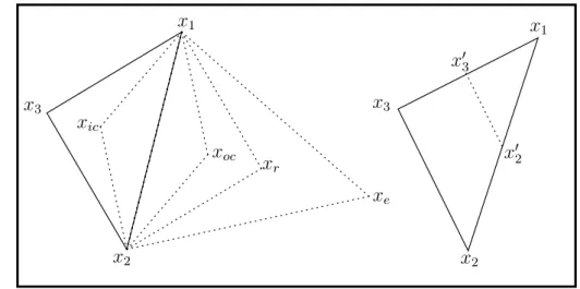
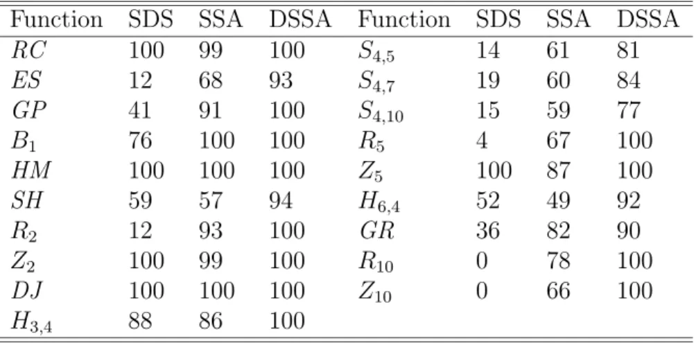
Table 2.1: Percentage of successful trials for SDS, SSA and DSSA Function SDS SSA DSSA Function SDS SSA DSSA
RC 100 99 100 S4,5 14 61 81
ES 12 68 93 S4,7 19 60 84
GP 41 91 100 S4,10 15 59 77
B1 76 100 100 R5 4 67 100
HM 100 100 100 Z5 100 87 100
SH 59 57 94 H6,4 52 49 92
R2 12 93 100 GR 36 82 90
Z2 100 99 100 R10 0 78 100
DJ 100 100 100 Z10 0 66 100
H3,4 88 86 100
functions with many crowded local minima such as Shubert function, functions with a global minimum lying in a very narrow hole such as Easom function, functions with a narrow valley such as Rosenbrock function, and smooth functions such as De Joung function and Zakharov function. For each function we made 100 trials with different starting points. The average number of function evaluations and the average error are related to only successful trials.
First, to demonstrate the effect of hybridizing simulated annealing with SDS to design SSA and DSSA, we show in Table 2.1 the percentage of successful trials. From Table 2.1, we see that the rate of success for SSA is generally better than that for SDS. However, the behavior of SDS for Zakharov functionZ5 is better than that of SSA due to the fixed cooling schedule in SSA for all functions. We note that the behavior of these methods has changed drastically when the dimension n of function Zn is increased to 10. Moreover, Table 2.1 clearly shows that the behavior of DSSA is the best of the three methods in terms of the rate of success.
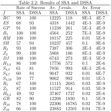
In Table 2.2, we show the effect of accelerating the cooling schedule in SSA and applying a local search method on the final results obtained by the accelerated SSA to design DSSA.
The results in Table 2.2 reveal that the acceleration procedure successfully affects the rate of success, the average number of function evaluations (Av. f-evals.), and the average error (Av. Error).
To show to what extent DSSA succeed in accelerating SA, we compare its results with other simplex SA method like SIMPSA and NE-SIMPSA [13]. Table 2.3 shows the average
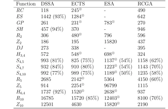
![Table 3.2: Average number of function evaluations in SCGA and other metaheuristics Function SCGA RCGA [11] CGA ⊗ [16] DSSA](https://thumb-ap.123doks.com/thumbv2/123deta/7309015.2421389/54.892.152.711.199.686/table-average-number-function-evaluations-scga-metaheuristics-function.webp)