Deep Learning Improving Learning Efficiency by Using Noise for Back Propagation
Kazuki NAGAO, Shinsaburo KITTAKA, Yoko UWATE and Yoshifumi NISHIO Dept. of Electrical and Electronic Engineering of Tokushima University 2-1 Minami-Josanjima, Tokushima-shi, Tokushima-ken 770-8506, Japan
Email: { k-nagao, kittaka, uwate, nishio } @ee.tokushima-u.ac.jp
Abstract—Deep learning began to be rapidly attention such as image recognition from the 2010. Now, the third time of artificial intelligence is boom. Deep learning is made to imitate the human nervous system. It automatically learns valid features of discrimination. That is why it is popular. In this study, we study about deep learning using noise for back propagation. Then, we improve the learning accuracy and reduce learning loops.
I. I
NTRODUCTIONHuman nervous system has neurons which are connected. It is controlled by the strength of neurons. Then, human can think things. Deep learning is made to imitate the human nervous system[1]. There are concepts and methods of deep learning from before and after 1980. It began to be rapidly attention such as image recognition from the 2010. Now, the third time of artificial intelligence is boom.
Deep learning is superposition of neural networks and has deep structure. Deep learning has more three layers include input layer and output layer. It is repeated learning by the time, and the input data is gradually being transferred to the deeper and deeper from the first layer. Previously, researchers and engineers had set the parameters manually. Now, that deep learning automatically learns valid features of discrimination.
It has been improved accuracy of pattern recognition. It is attracting attention.
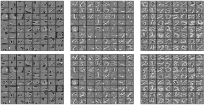
Fig. 1. Recognition of numbers by deep learning.
In June 2012, it was able to recognize the cat on computer by research of Google. After that, it came to be used in
various fields. For example, image field, emotional awareness, module of self-driving, medical field, financial field and so on... Google released a software library of machine learning techniques including deep learning in 2015, and we raised interest in deep learning. Figure 1 shows recognition of numbers by deep learning with Google’s software library[2].
In deep learning, there is a variety of techniques in order to improve the learning accuracy. Technique of back propagation compares input data and output data to find deviations of feature values and optimize weights. This technique can reduce learning loops. If the learning period is too long or the training data is not typical, it adapts to features unrelated to the features that should be originally learned. This phenomenon is called over learning. In such a case, it is used the method of dropout to correspond to input data. Deep learning requires a large amount of learning data. When there is not too much input data, input data is shifted slightly due to use noise to increase features. There are various techniques like these.
In this study, we propose new system of deep learning. This system is noisy feed back. Weights of neurons are optimized using a noise in the back propagation. Purposes of this study are to improve learning accuracy and to reduce learning loops.
There are two patterns which are a small deep learning model (A) and a deep learning model (B). We compared conventional system and two patterns of proposed system.
1II. P
ROPOSED METHODFigs. 2 and 4 show conventional system. Figs. 3 and 5 show proposed system. Arrows of left to right indicate propagation of input signal and right to left indicate learning of back propagation.
(A) Iris data set
We use a model consisting of two layers of intermediate layers and Gaussian distribution (0, 0.01) for noise and add it to equations (2). In addition, the putting place of Gaussian distribution (0, 0.01) is changed. We experiment 8 patterns about conventional system without noise, (h
1back), (h
2back), (y
back), (h
1back, h
2back), (h
1back, y
back), (h
2back, y
back) and (h
1back, h
2back, y
back). These combinations indicate where noise is added.
1This research is that we add one dataset to what was announced at SJCIEE.
- 1 -
IEEE Workshop on Nonlinear Circuit Networks December 9-10, 2016
Fig. 2. Schematic drawing of deep learning consisting of two intermediate layers.
Fig. 3. Schematic drawing of proposed deep learning consisting of two intermediate layers.
h
1= 1 1 + e
(−∑
w1x)h
2= 1 1 + e
(−∑
w2h1)y = 1
1 + e
(−∑
(w3h2))(1)
y
back= (y − ty)(1 − y)y h
2back= ∑
w
3y
back(1 − h
2)h
2h
1back= ∑
w
2h
2back(1 − h
1)h
1(2)
w
1(l+1)= w
1l− εxh
1backw
2(l+1)= w
2l− εh
1h
2backw
3(l+1)= w
3l− εh
2y
back(3)
ε is the rate of decay which is 0.01. h means activation function. w means weights between neurons. The initial value of the weights is chosen by random from 0.04 or less.
(B) Cars data set
We use Gaussian distribution (0, 0.01) for noise and add it to equations (5). In addition, the putting place of Gaus- sian distribution (0, 0.01) is changed. We experiment 15
patterns about conventional system without noise, (h
1back), (h
2back), (h
3back), (y
back), (h
1back, h
2back), (h
1back, h
3back), (h
1back, y
back), (h
1back, h
2back, h
3back), (h
1back, h
2back, y
back), (h
1back, h
3back, y
back), (h
1back, h
2back, h
3back, y
back), (h
2back, h
3back), (h
2back, y
back), (h
2back, h
3back, y
back) and (h
3back, y
back). These combinations indicate where noise is added.
Fig. 4. Schematic drawing of deep learning consisting of three intermediate layers.
Fig. 5. Schematic drawing of proposed deep learning consisting of three intermediate layers.
h
1= 1 1 + e
(−∑
w1x)h
2= 1 1 + e
(−∑
w2h1)h
3= 1 1 + e
(−∑
w3h2)y = 1
1 + e
(−∑
(w4h3))(4)
y
back= (y − ty)(1 − y)y h
3back= ∑
w
4y
back(1 − h
3)h
3h
2back= ∑
w
3h
3back(1 − h
2)h
2h
1back= ∑
w
2h
2back(1 − h
1)h
1(5)
w
1(l+1)= w
1l− εxh
1backw
2(l+1)= w
2l− εh
1h
2backw
3(l+1)= w
3l− εh
2h
3backw
4(l+1)= w
4l− εh
3y
back(6)
ε is the rate of decay which is 0.4. h means activation function. w means weights between neurons. The initial value of the weights is chosen by random from 0.3 or less.
- 2 -
III. S
IMULATION RESULT(A) Iris data set
Learning accuracy and learning loops are better to be smaller. We define as the learning loops = 25000 and the number of learning data sets = 150.
Figure 6 shows change of the learning accuracy and learning loops of conventional system and proposed system. Table I shows learning accuracy for all kinds of patterns. Table II shows learning loops when learning accuracy is 0.15 or less.
From Figure 6, the learning accuracy and learning loops of using Gaussian distribution (0, 0.01) are better than not using it. From Table I, most results by using the noise are found to be better.
Fig. 6. Simulation results of schematic drawing of deep learning consisting of two intermediate layers.
TABLE I
LEARNING ACCURACY OF MODEL(A).
accuracy Conventional 0.1771
h1back 0.1787
h2back 0.1727
yback 0.0269
h1backh2back 0.1750 h1backyback 0.0178 h2backyback 0.1708 h1backh2backyback 0.0261
TABLE II
LEARNING LOOPS OF MODEL(A).
loops
yback 12612
h1backyback 8002 h1backh2backyback 11103
(B) Car data set
Learning accuracy and learning loops are better to be smaller. We define as the learning loops = 1000 and the number of learning data sets = 1728.
Figure 7 shows the learning accuracy and learning loops of conventional system and proposed systems. Table III shows learning accuracy of minimum value and average for all kinds of patterns. Table IV shows learning loops for all kinds of patterns when learning accuracy is 0.07 or less.
From Figure 7, the learning accuracy and learning loops of using Gaussian distribution (0, 0.01) are better than not using it. From Table IV, h
2backy
backand y
backare better than conventional about minimum value and average value.
Fig. 7. Simulation results of schematic drawing of deep learning consisting of three intermediate layers.
TABLE III
LEARNING ACCURACY OF MODEL(B).
minimum average
Conventional 0.052 0.0634
h1back 0.060 0.0734
h2back 0.057 0.0697
h3back 0.064 0.0639
yback 0.050 0.0591
h1backh2back 0.060 0.0667
h1backh3back 0.058 0.0702
h2backh3back 0.056 0.0723
h1backh2backh3back 0.057 0.0650
h1backyback 0.054 0.0660
h2backyback 0.049 0.0595
h3backyback 0.057 0.0718
h1backh2backyback 0.052 0.0707 h1backh3backyback 0.053 0.0678 h2backh3backyback 0.054 0.0738 h1backh2backh3backyback 0.054 0.0724
TABLE IV
LEARNING LOOPS OF MODEL(B).
loops
Conventional 29
h1back 11
h2back 84
h3back 6
yback 2
h1backh2back 6
h1backh3back 76
h2backh3back 46
h1backh2backh3back 10
h1backyback 45
h2backyback 2
h3backyback 39
h1backh2backyback 221 h1backh3backyback 8 h2backh3backyback 5 h1backh2backh3backyback 13
- 3 -
IV. C
ONCLUSIONIn this study, we proposed new technique of deep learning. It is using noise at back propagation. In the proposed technique, we choose gaussian distribution (0, 0.01) for noise. Then, we examined whether this technique is effective in simulation that is using two data sets.
In simulations, we were able to improve learning accuracy and reduce learning loops to use noise at back propagation.
From the tendency of research results of two data sets, we found that results are improved by using noise at back propa- gaion from the output layer to the final intermediate layer.
Because back propagation of the output layer is compared with input data and output data, so it is properly carried out weight adjustment.
In the future work, we use other data sets to demonstrate usability and a variety of noise. Then, we obtain the good performance of the proposed technique.
A
CKNOWLEDGMENTThis work was partly supported by JSPS Grant-in-Aid for Challenging Exploratory Research 26540127.
R
EFERENCES[1] Chihiro Ikuta, Yoko Uwate and Yoshihumi Nishio, ”Investigation of Be- havior of Deth of Neuron and Neurogenesis in Multi-Layer Perceptron,”
2013 IEEE Workshop on Nonlinear Circuit Networks, pp. 65-68, 2013 [2] Dumitru Erhan, Yoshua Bengio, Aaron Courville, Pierre-Antoine Man- zagol, Pascal Vincent, Samy Bengio, ”Why Does Unsupervised Pre- training Help Deep Learning?,” Journal of Machine Learning Research 11, pp. 625-660, 2010
[3] Shohei Gotoda, Yoko Uwate and Yoshihumi Nishio, ”Cellular Neural Networks with Changing Templates for Image processing,” 2015 IEEE Workshop on Nonlinear Circuit Networks, pp.21-23, 2015
[4] Shinsaburo Kittaka, Ryota Oshima, Yoko Uwate and Yoshifumi Nishio,
”Feed-forward Neural Netwotks with Changing Sigmoid Functions,”
Journal of Shikoku-Section Joint Convention of the Institutes of Elec- trical and Related Engineers, No.1-27, p.27, 2015