その他のタイトル
(材料特性の不確定性の定量化とその応用)
著者
SH
AH
I N
U
R SW
EETY
学位名
博士(工学)
学位授与機関
北見工業大学
学位授与番号
10106甲第166号
研究科・専攻名
生産基盤工学専攻
学位授与年月日
2018- 03- 16
Thesis
Quantification of uncertainty of material
properties and its application
March 2018
Doctoral Thesis
Quantification of uncertainty of material
properties and its application
i
List of Contents
List of Contents ... i
List of Figures ... vii
List of Tables ... xiii
Abstract ... xv
Chapter 1: Introduction ... 1
1.1 General Background ... 1
1.1.1 Materials and their Properties ... 1
1.1.2 Sustainability ... 3
1.1.3 Uncertainty ... 6
1.1.4 Uncertainty in Material Selection ... 10
1.1.4.1 Uncertain Material Properties ... 10
1.1.4.2 Uncertainty in MI Calculation ... 11
1.1.4.3 Uncertainty in MI Method ... 12
1.1.5 Objectives or Requirement ... 13
1.2 Core Idea/ How to Deal with Different Uncertainties ... 14
1.2.1 Uncertainty Quantification ... 14
1.2.2 Tool for Material Selection ... 15
1.2.3 Compliance ... 16
1.3 Scope of the Work ... 21
1.4 Objectives of the Work ... 21
ii
1.6 Thesis Structure ... 27
Chapter 2: Mathematical Settings ... 31
2.1 Probability Distribution ... 31
2.2 Average, Standard Deviation and Ranges of Mean and Variance ... 34
2.3 Possibility Distribution or Fuzzy Number ... 35
2.3.1 Trapezoidal Fuzzy Number ... 38
2.3.2 Triangular Fuzzy Number ... 38
2.3.3 Ramp Up Fuzzy Number ... 39
2.3.4 Ramp Down Fuzzy Number ... 40
2.4 Degree of Compliance ... 41
2.4.1 Degree of Compliance of Crisp Value ... 42
2.4.2 Degree of Compliance of Crisp Granular Value or Range ... 43
2.4.3 Degree of Compliance of Triangular Fuzzy Number/ Possibility Distribution ... 45
2.4.3.1 Interaction of D with MAX ... 46
2.4.3.2 Interaction of D with MIN ... 48
2.5 Induction of Fuzzy Number ... 49
Chapter 3: Uncertainty Quantification of Mechanical Properties of Jute Yarn 59 3.1 Mechanical Properties ... 59
3.1.1 Tensile Strength and Modulus of Elasticity ... 60
3.1.2 Density ... 61
3.2 Sustainable Properties ... 61
3.2.1 CO2 Footprint ... 61
iii
3.2.3 Water usage ... 62
3.3 Production of Jute Material ... 62
3.4 Description of Experiment ... 63
3.5 Results... 66
3.5.1 Mechanical Properties ... 66
3.5.2 Uncertainty in the Mechanical Properties ... 67
3.6 Uncertainty Quantification ... 68
3.6.1 Uncertainty Quantification by Statistical Method ... 69
3.6.2 Uncertainty Quantification by Probabilistic Method ... 70
3.6.2.1 Parameter Calculation ... 71
3.6.3 Uncertainty Quantification by Possibilistic Method ... 76
3.6.4 Comparison among the Different Methods ... 78
3.7 Conclusion ... 83
Chapter 4: Decision Model to Select a Material under Uncertainty ... 87
4.1 Epistemic Uncertainty in Product Development ... 87
4.2 Mathematical Description of the Model ... 90
4.2.1 Formulation Module ... 91
4.2.2 Information Gathering Module ... 92
4.2.2.1 Determining the Supports ... 92
4.2.3 Compliance Calculation Module ... 94
4.2.4 Aggregation Module ... 94
4.2.5 Decision Module ... 96
4.3 Implication of the Model: A Case Study ... 96
iv
Chapter 5: Discussions ... 111
Chapter 6: Concluding Remarks ... 131
List of References ... 137
List of Research Achievements ... 157
Acknowledgments ... 161
vii
List of Figures
viii
Figure 2.1:Weibull (a) density function and (b) cummulative distribution for
different shape and scale factor. ... 32
Figure 2.2: A typical nature of fuzzy number. ... 36
Figure 2.3: Different shapes of the fuzzy numbers(a) triangular (b) ramp up (c) Ramp down and (d)trapezoidal. ... 37
Figure 2.4: Trapezoidal fuzzy number. ... 38
Figure 2.5:A triangular fuzzy number. ... 39
Figure 2.6: (a) Ramp up and (b) typical pattern of ramp up function. ... 40
Figure 2.7: (a) Ramp down and (b) typical pattern of ramp down function. ... 40
Figure 2.8: Interaction between crisp value and (a) MAX and (b) MIN fuzzy numbers. ... 43
Figure 2.9: Interaction between crisp granular value and (a) maximization and (b) minimization fuzzy number. ... 44
Figure 2.10: A typical nature of (a) RCMAX and (b) RCMIN. ... 45
Figure 2.11: (a) Interaction between the triangular and maximization fuzzy numbers and (b) A typical nature of TCMAX. ... 46
Figure 2.12: (a) Interaction between a triangular and a minimization fuzzy number and (b) Typical nature of TCMIN. ... 48
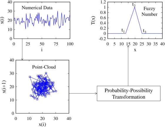
Figure 2.13: Representing the uncertainty of numerical data using a triangular fuzzy number. ... 50
Figure 2.14: A given set of numerical data. ... 51
Figure 2.15: Relative position of A and B in the point-cloud (x(t), x(t+1)). ... 52
Figure 2.16: (a)The typical nature of PrA(x) and PrB(x) for unimodal quantity and (b) Nature of PrA(x)+PrB(x) and min(PrA(x),PrB(x)) for unimodal data ... 53
ix
Figure 2.18: The nature of (a) probability (b) possibility distribution of a
unimodal point-cloud. ... 55
Figure 2.20: Numerical data to Possibility distribution transformation. ... 57
Figure 3.1: Data analysis of stress-strain curve for (a) linear and (b) non-linear. ... 60
Figure 3.2: Primary production jute yarn. ... 63
Figure 3.3: Schematic diagram of the experiment ... 64
Figure 3.4: (a) Experimental equipment and (b) Gripping. ... 65
Figure 3.5: Magnified (a) front and (b) cross section view of yarn specimen. ... 65
Figure 3.6: Load versus elongation plots of fifteen jute yarn specimens. ... 66
Figure 3.7: Uncertainty in the mechanical properties (a) TS, (b) E, and (c) s of the jute yarn. ... 68
Figure 3.8: Estimation of Weibull parameters. ... 72
Figure 3.9: ln(ln(1/1-F (xi))) - ln(x) plot for (a) TS, (b) E, and (c) s of jute yarn. 73 Figure 3.10: Least mean square line plots of (a) TS,(b) E, and (c) s for the jute yarn. ... 73
Figure 3.11: Weibull density functions of the (a) TS, (b) E, and (c) s for jute yarn. ... 75
Figure 3.12: Possibility distribution of (a) TS, (b) E, and (c) s of jute yarns. ... 76
Figure 4.1: A scenario of epistemic uncertainty regarding a material selection of a product vehicle. ... 88
Figure 4.2: Schematic diagram of the decision making procedure under uncertainty. ... 89
Figure 4.3: Proposed decision model. ... 90
x
Figure 4.5: Decision-relevant information for three different categories of metal alloys. ... 99 Figure 4.6: Objective functions of six criteria. ... 100 Figure 4.7: Interaction between crisp granular information with the objective function for Al 2014, wrought T4 alloy. ... 101 Figure 4.8: Compliances of the alternatives for a respective criterion. ... 102 Figure 4.9: Possibility distribution of the alternatives for the respective criterion. ... 102 Figure 4.10: Interaction between the objective function and the possibility distribution for five criteria, three alternatives. ... 104 Figure 5.1: A Complete framework of eco-product development. ... 112 Figure 5.2: Jute product made from jute yarn. ... 114 Figure 5.3: Comparison between jute fiber and yarn in terms of uncertainty in TS
xi
xiii
List of Tables
Table 1-a. Data of the material properties of A and B for tie regarding MI. ... 11
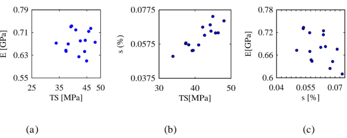
Table 3-a. Mechanical properties of jute yarn. ... 67
Table 3-b. Statistical uncertainties of jute yarn. ... 69
Table 3-c. Indexing of the TS, E, and s data for jute yarn. ... 71
Table 3-d. Weibull parameters for TS, E, and s of jute yarn. ... 74
Table 3-e. Probabilistic uncertainties (Weibull distribution) of jute yarn. ... 75
Table 3-f. Possibilistic parameters of jute yarn. ... 77
Table 3-g. Probabilistic and possibilistic uncertainties of jute yarn. ... 79
Table 3-h. Error estimation of quantified data for mechanical properties of jute yarn. ... 82
Table 4-a. List of Alternatives (Ai| i = 1,…,3). ... 97
Table 4-b. States of Criteria and their supports. ... 99
Table 4-c. Ranking scores of the alternatives. ... 105
xv
Abstract
xvi
xvii
1
Chapter 1:
Introduction
The notion of uncertainty has earned a great deal of attention from the researchers belonging to various academic disciplines. In this study, the uncertainty in the material properties is considered and its application, particularly, the material selection for developing a product has been investigated. The remainder of the chapter is structured as follows: General Background, Core Idea, Scope, Objectives, Literature Review, and the Thesis Structure.
1.1General Background
Engineering materials and their properties, the concept of sustainability, uncertainty and their categories, uncertainties in product development particularly material selection are described in this subsection.
1.1.1 Materials and their Properties
2
know how to select the optimal materials for each component mentioned in the above, from a large number of alternatives.
Figure 1.1: Dependency of a product on different elements.
In 1945, there were only four categories of engineering materials, namely, Metals and Alloys, Polymers and Elastomers, Ceramics and Glasses, and Natural Materials. Now, there are two more categories, namely, Foams and Composites, resulting more than 80,000 members in the Universe of Materials. Refer to (Mousavi-Nasab and Anvari, 2017) and (Ashby, 2007) for more details regarding the types of materials. Therefore, material selection is a difficult problem to solve. Usually, the material is selected using a function called Material Index, MI (Ashby, 2007). The material selection procedure is briefly described as follows.
Consider an object schematically shown in Figure 1.2. Depending on the shape, support, and loading condition, it can be considered a Column, Plate, Tie, Beam, or Panel or any combinations. It is made from a material, which has different properties such as mechanical, chemical, optical, thermal, sustainable, electrical, magnetic, atomic, and manufacturing properties.
Product Component handle
zipper chamber
Shape Material
Function
3
Figure 1.2: Schematic diagram of a mechanical object under load and torque.
From the sustainable manufacturing point of view for a mechanical object along with other material properties, sustainable properties are important. In this study, mechanical and sustainable properties are emphasized. The mechanical properties include tensile strength (TS), modulus of elasticity (E), hardness, density (ρ), endurance limit (σe), fracture toughness, and compressive strength.
On the other hand, the sustainable properties (Ashby, 2007) include Carbon dioxide (CO2) Footprint, Water usage, Recycle fraction, Cost, Reservation, Safety, and Environmental damage. Consider a case, to select materials for a mechanical object ‘tie’. Nowadays, while selecting materials, the sustainability is taken as one of the key considerations by engineers and researchers. The idea of sustainability is described in the following section.
1.1.2 Sustainability
In this section, the concept of sustainability is enhanced. Sustainability means fulfilling the present-day needs without jeopardizing the potential of fulfilling the future needs (N.N, 1987; Ullah, et al., 2014). The salient point of sustainability is schematically illustrated in Figure 1.3. As seen in Figure 1.3, two worlds, artificial (marked as 1) and natural worlds (marked as 2), simultaneously exist around us, and they must be synergistic to each other. The concept of ‘sustainability’ deals with issues related to the coexistence of natural and artificial worlds (Umeda, et al., 2009; Ullah, et al., 2017). In particular, the natural world consists of natural resources (water, air, land, ore, biomass, and
F
F M
F
F
Column
Plate
Tie
Beam
4
hydrocarbon) whereas the artificial world consists of products (car, road, building, plane, train, pen, computer, paper, and many more). Using the natural resources, primary energy and materials are produced. Afterward, the primary energy and materials are used to produce products and support their lifecycles (marked as 4). The artificial world is full of man-made products; each product has a life cycle. A lifecycle means the chronological stages of a product, namely, conceptualization, design, manufacturing, use, recycle, and landfill. To obtain primary materials and energy, resources (marked as 3) are required which are obtained from the natural world. If a product (or its lifecycle) needs a large amount of energy and materials, it puts burden on the natural resources, and, thereby, on the natural world. This means the natural world is exhausted to enrich the artificial world by producing and maintaining products.
Figure 1.3: The concept of the life cycle from the viewpoint of the primary energy.
This means that the sustainability is jeopardized if the demands of primary energy and materials are not kept within the stipulated limits. Numerous studies have shown that the types and usages of materials in the products (i.e., the constituents of the artificial world) heavily affect the sustainability (Ullah, et al., 2014; Ullah, et al., 2013; Shahinur and Ullah, 2017). However, for
Sustainability
Artificial World Natural World
Product and their Lifecycles
Water, Air, Land, Ore, Biomass,
Hydrocarbon
Primary Materials/Energy Conceptualization
Design Manufacturing Use
Recycling/Disposal Landfill
4
1 2
5
sustainability, both these worlds must coexist, and we must not overburden the natural world as well as fulfill the needs of the artificial world.
Many strategic goals have been set to achieve sustainability of the environment, one important goal is to reduce the global CO2 Footprint by half, by the year
2050 (Allwood, et al., 2010) schematically shown in Figure 1.4.
Figure 1.4: Important strategy to maintain the sustainability.
Effective CO2 reduction requires the simultaneous attainment of efficiency in terms of materials, energy, and components of products (Allwood, et al., 2010; Milford, et al., 2013; Allwood, et al., 2011; Ullah, et al., 2013; Ullah, et al., 2014). Improving material efficiency means increasing the use of environmental friendly materials, increasing material yields, and making lightweight products (Allwood, et al., 2010; Milford, et al., 2013; Allwood, et al., 2011; Ullah, et al., 2013; Ullah, et al., 2014). Energy efficiency denotes deploying renewable energy sources, and decreasing energy usage (Ullah, et al., 2013; Ullah, et al., 2014). It has been found that material efficiency is more effective than energy efficiency in achieving the strategic goals of sustainability (Allwood, et al., 2010; Milford, et al., 2013; Allwood, et al., 2011; Ullah, et al., 2013; Ullah, et al., 2014). One of the options for achieving material efficiency is to increase the amount of usage of natural materials in various products as much as possible (Alves, et al., 2010). The natural materials have low density as schematically shown in Figure 1.5 and require low energy for the primary material productions. Thus, natural materials are better option for sustainability of the product compared to other materials.
100%
50% Recycle, energy mix, energy efficiency
Reduction/diversification of material usages
2050 Now
6
Figure 1.5: Importance of natural materials on the view point of eco-product (Ashby, 2007).
In this study, a widely used natural material, ‘jute’ has been selected, which grows mainly in Bangladesh, India, and China (Anon., 2017). The motivation behind selecting the jute fiber is due to their abundant availability in the nature followed by cotton and bamboo (Barth and Carus, 2015). It is a natural fibrous material having good mechanical (Xia, et al., 2009), thermal (Pandey, et al., 1993), and sustainable properties. For instance, jute exhibits excellent weight per strength ratio compared to the metal. Many researchers have gained interest in jute for the sustainable product due to its biodegradable and nontoxic nature. However, the knowledge of the natural material is uncertain to take a decision on the eco-product manufacturing. The concept of uncertainty is explained in the following section.
1.1.3 Uncertainty
Uncertainty is often understood (semantics) by classifying it into different categories, (Booker and Ross 2011; Ross et al., 2013) as follows:
a) Aleatory uncertainty,
b) Epistemic uncertainty,
Metals
Cera
m
ic
s
Pol
ym
ers
an
d
el
ast
om
ers
Density, ρ
T
ens
il
e
St
ren
g
th
,
T
S Eco-friendly materials
High density and high strength means less
7
c) Reducible uncertainty,
d) Irreducible uncertainty, and
e) Inference uncertainty
In general, aleatory uncertainty refers to uncertainty due to random variability or stochastic processes. In case of aleatory uncertainty, distribution is known at the beginning and the data vary due to that distribution as schematically illustrated in Figure 1.6(a).
Figure 1.6: The variability of data due to different uncertainties.
Epistemic uncertainty refers to uncertainty due to lack of knowledge or imprecision associated with the data and information. In case of epistemic uncertainty, it is not known which distribution data will follow as shown in Figure 1.6(b). The possibility distribution is generally used to quantify the epistemic uncertainty and it is the neutral representation of the uncertainty (Ullah and Shamsuzzaman, 2013; Ullah, 2016). The mathematical procedure related to this distribution is described in Appendix-A.
Reducible uncertainty refers to the uncertainty that can be reduced by applying different conditions as shown in Figure 1.6 (c). Irreducible uncertainty refers to
?!
Aleatory
Epistemic
Reducible
Irreducible
Inference A change in
the system
Pro
b
(x
)
x
Samples
Samples Samples
Samples Samples
Samples
Samples
A change in the system
x
x
x
x
x
x
Pro
b
(x
)
Samples
Samples
Samples a
b
c
d
8
uncertainty due to natural variability that can be quantified but cannot be reduced. In such case, the variability or uncertainty in the data cannot be reduced or controlled by physical means (for example chemical modification, x-ray, and radiation) as shown in Figure 1.6 (d).
Inference uncertainty refers to predicting the future from the past, inferring the population behavior from a sample, and inferring the system behavior from its subsystems. In such case, infinite estimation can be made from finite world as shown in Figure 1.6 (e).
To compute uncertainty in a formal manner (syntax), theories have been developed, for example, probability theory, imprecise probability theory, evidence theory, possibility theory, and random interval theory (Dempster, 1968; Walley, 1991; Walley 2000; Shafer, 1976; Klir, 1990; Zadeh, 1978; Dubois and Prade, 1988; Joslyn and Booker, 2004). In certain cases, the theories are based on different categories of uncertainty. For example, the probability theory deals mainly with the aleatory uncertainty, whereas the possibility theory deals with the epistemic uncertainty. Certain theories can deal with multiple categories of uncertainty, e.g., imprecise probability theory can deal with aleatory uncertainty and the epistemic uncertainty associated with the probabilities of events. Nevertheless, the uncertainty of a category can be interpreted in terms of the uncertainty of a different category as schematically shown in Figure 1.7 (Klir, 1999; Dubois et al., 2004; Ullah and Shamsuzzaman 2013).
9
Figure 1.7: One types of uncertainty can be transformed into other uncertainty.
Again, when the distribution of reducible and irreducible uncertainty is not known, they become as epistemic uncertainty marked as 3 as schematically shown in Figure 1.7 As it is discussed before the epistemic uncertainty can be quantified by using previously mentioned theory. Moreover, if the distribution is known (probability distribution) they are named as aleatory uncertainty and can be quantified using probability theory as shown in Figure 1.7 marked as 4. That means the aleatory uncertainty, epistemic uncertainty, and any other uncertainty are different from each other in the sense of semantics, but all these uncertainties are somewhat same in the computational science, and, thereby, can be integrated while developing systems for making decisions under uncertainty irrespective of its category. There is uncertainty regarding the material selection method, MI, is discussed below.
X
Poss
(
X
)
70 85 100 115 130 0 0.25 0.5 0.75 1 Reducible Epistemic Inference Inference
䐟
䐠 䐠
䐡 䐡
X Pro b (X )/ Po ss (X )
50 100 150
0 0.25 0.5 P ro b ( X )
70 85 100 115 130 0 0.25 0.5 0.75 1 1 0.75 X 4 Aleatory Samples X
0 4 8 12 16 20 60 80 100 120 140 Samples X
0 4 8 12 16 20 60
10
1.1.4 Uncertainty in Material Selection
Material is an important issue for a component of the product and needs to be considered in selecting material. Thus, to select a material for an object from the Material Universe, it is required to differentiate one material from other materials. Usually, to select a material for a component of the product, a function termed as, MI, (Ashby, 2007) is used. The general formula for MI
(particularly for stiffness and strength limited design for an object) is given by equation (1.1).
c b a
E
TS
MI
(1.1)The MI is related to three mechanical properties, namely TS, E and ρ which are important in selecting a material. In case of optimal material selection, the maximum value of the MI should be considered (Ashby, 2007). For example, if a tie is considered, it will bear only tensile load and the values of the exponentials of the equation (1.1) are a = 1, b = 0, and c = -1. Therefore, the MI
(one types of knowledge) for tie can be defined using the equation (1.2) (Ashby, 2007).
TSMI
(1.2)There are uncertainties in selection of materials using MI. These issues are discussed in next section.
1.1.4.1Uncertain Material Properties
11
required. The mechanical properties of the tie are determined through the tensile test, by applying the tensile load on a sample. Thereafter calculation, the results of TS and ρ are found. The procedure is repeated for different samples. The experimental results vary from sample to sample. Therefore, it can be inferred that there is uncertainty in the data of material properties. As the data of material properties are uncertain, it is tough to judge a material according to MI.
Table 1-a. Data of the material properties of A and B for tie regarding MI.
Material
Properties
TS ρ �� = ⁄�
A 300 100 3
B 200 50 4
1.1.4.2Uncertainty in MI Calculation
There is uncertainty in the MI itself. Suppose, there is a ‘Table’ (as shown in
Figure 1.8) where the top of the ‘Table’ is considered as a plate, two sides of the ‘Table’ are considered as column and base of the ‘Table’ is considered as a beam. That means a product is a combination of multiple components. Moreover, the MI of each component is different. Though the MI of the column
( ), beam ( ) and plate ( ) (Ashby, 2007) are known, however, it is difficult to know what will be the MI of the ‘Table’.
Figure 1.8: A mechanical object (‘Table’) is a combination of multiple components.
Plate
Beam
Col
12
Generally, the shapes of the mechanical components are more complex. Therefore, it is difficult to calculate the MI of the complex shape. Therefore, MI
itself is uncertain or cannot be derived. Even though MI can be calculated for the different machine elements, MI cannot be calculated for a given product. As MI
is uncertain, an alternative option for selecting material is required.
1.1.4.3Uncertainty in MI Method
There is uncertainty in the material selection using MI method. Consider the material selection procedure using MI, from the Material Universe, for a mechanical object ‘tie’. As discussed in the previous section, MI of a tie is the ratio of TS and ρ. Now if the straight line is drawn in the engineering Material Universe plot as schematically shown in Figure 1.9, the value of the slope of the straight line will represent the MI of the tie.
Figure 1.9: Various types of materials under same slope line (Ashby, 2007).
The equation of straight line is = + , where x = ρ, y = TS, m = MI, and c
= 0. To select an optimal material, MI should always be maximized. From Figure 1.9, it can be informed that the materials which lie on MI = 1 are better material than those having MI = 0.1 and MI = 0.01. All materials correspond to a single slope line, say M1, M2, and M3 of MI are equivalent. That means there are
Metals
Ceram
ic
s
Po
ly
m
ers
an
d
elast
o
m
ers
ρ
T
S
MI= 1
MI= 0.1
MI = 0.01
13
many good materials which can be selected for a tie under MI =1 alone. Now, which good material can be selected for the tie? It is difficult to choose a material for the tie even though the MI is known. Therefore, it can be inferred that MI does not guarantee the selection of a single material.
From the above description, it is clear that there is uncertainty, (epistemic), in the data of material properties, uncertainty in the MI. When MI is uncertain it cannot give a guarantee of a single material selection. Thus, it is hard to compare one material with another and to make the list of preference of materials. Furthermore, sustainable properties cannot be incorporated in the material selection procedure under MI. Therefore, it is essential to deal and manage these types of uncertainty to ensure the selection of material for the sustainable product. Furthermore, what will be the tool to deal these types of uncertainties? It is an important issue.
1.1.5 Objectives or Requirement
At the early stage of the product development, objectives are partially known. These objectives are the customer requirements and it is referred as ‘zero stage’ of a solution. For example, if a strong material is required then objective is to have a material with high TS. For structural integrity, TS and ρ are needed to be maximized and minimized, respectively. For sustainability, CO2 Foot print, Water usages, Environmental damage are needed to be minimized whereas the
14
1.2Core Idea/ How to Deal with Different Uncertainties
This section describes the core idea to deal with uncertainty of the material properties, uncertainty in the MI regarding the selection of material.
1.2.1 Uncertainty Quantification
As described in Section 1.1.4.1 the raw data of material property (for example
TS) is not a single value and it varies a lot. In this study, this type of variation in material property means a kind of uncertainty, so material cannot be selected based on this uncertainty. Therefore, quantification and maintenance of the uncertainty for selection of material is a vital issue. Quantification of the uncertainty can be done by different approaches. Through literature review, it is found that three quantification approaches such as statistical, probabilistic and possibilistic are most widely used. The quantified data of the material properties can be represented by statistical range or probabilistic form or possibilistic form as schematically shown in Figure 1.10. From these three methods which one will be used for uncertainty quantification and which is reliable method to quantify the uncertainty, is an important issue. In this study, a reliable approach to quantify the uncertainty is investigated.
Figure 1.10: Quantification of the uncertainty using three approaches.
Raw Data of Material Properties
Statistical Method
Probabilistic Method
15
1.2.2 Tool for Material Selection
At the initial stage of product development, MI is unknown and objectives are partially known. As the information is not known or partially known, they can be represented by a fuzzy function. In this study, two types of possibility objective functions have been proposed, namely, maximization and minimization as shown in Figure 1.11. Possibility Objective function is selected based on requirement and common sense. The maximization function will be selected, when a high value of a criterion (say TS) is required as schematically depicted in Figure 1.11(a) and vice versa.
(a) (b)
Figure 1.11: Conflicting objectives representation by (a) Maximization and (b) Minimization function
The membership value of the possibility objective function lies between 0 and 1. Therefore, to build the objective function one must consider the range of x-axis, named as support. The support as shown in Figure 1.11 is derived from the Material Universe. It may be local, semi-local, deterministic or global (detail in Chapter 2). If minimum and maximum values of a property are plotted, support will be the range of the valuesof the x-axis.
Suppose designer’s objective is to have a strong as well as light material for a product (like a vehicle body). There are two objectives in designer requirements, such as strong material and light material. High TS is required for strong material and low ρ is required for light material. Therefore, for strong
D
o
B
(
T
S
)
TS
For strong material
Objective = maximize TS
1
0
Support DoB
(
ρ
)
ρ For light material
Objective = minimize ρ 1
0
16
material, TS needs to be maximized whereas, for light material, ρ needs to be minimized. Thus, the objective function for TS will be maximization function as shown in Figure 1.11(a). However, the objective function for ρ will be minimization function as shown in Figure 1.11(b). In Figure 1.11 x-axis represents the TS andρ, y-axis represents the degree of belief (DoB).
1.2.3 Compliance
17
(a) (b)
Figure 1.12: Compliance between material properties and (a) maximization and (b) minimization function.
It is assumed that there are two materials A and B and their corresponding degree of believe (DoB) for TS are 0.8 and 0.4, respectively as shown in Figure 1.12(a). It can be inferred that material A is a better option than B for strong material. Similarly, for light materials selection, the objective is to minimize the
ρ which can be represented in Figure 1.12(b). From Figure 1.12(b), it can be inferred that B material (DoB = 0.7) is better than A for a lighter material. Therefore, a strong, as well as light material can be selected using possibility distribution function without MI. Thus, using the possibility objective function one can represent ones feeling. Furthermore, one can also represent one’s requirement through these types of functions. Using compliance one can make a ranking of the materials and finally, can select a single material for product development. Therefore, MI can be replaced by Compliance calculation between the possibility objective function and the data of material property (or criteria). It can be said that it is an alternative representation of the MI.
However, when the data of the material properties is uncertain, the compliance calculations are different. According to literature, the uncertainty can be represented by statistical range, probabilistic form, and possibilistic form. In the previous example of Section 1.2.2, the two requirements are represented by two
A
D
o
B
(
T
S
)
TS
For strong material
Objective = maximize the TS
B 0.8
0.4 1
0 A
D
o
B
(
ρ
)
ρ For light material
Objective = minimize ρ
B 0.7
0.3 1
18
objectives functions, minimization, and maximization, as shown in Figure 1.11. Let, the uncertainties of material properties (TS and ρ) are represented by possibility distributions as shown in Figure 1.13. To obtain a strong material between A and B, interaction is required between the maximization objective functions (Figure 1.13(a)) and the possibility distributions of TS for corresponding materials.
(a) (b)
Figure 1.13: Compliance between (a) maximization and (b) minimization function uncertain (possibility distribution) material properties.
Now, if the values of compliances of two materials A and B for TS are 0.75 and 0.39, respectively, it can be inferred that material A is a better option than B for strong material. Similarly, for light materials selection, the objective is to minimize the ρ which can be represented in Figure 1.13(b). Let the values of compliance of A and B are 0.4 and 0.85, respectively. Thus, it can be inferred that material B is better than A for a lighter material based on the calculated compliances values.
Similarly, when the uncertainty of the data is represented by statistical range the interaction between the objective function and the uncertain data for ρ and TS
are shown in Figure 1.14. For this type of uncertainty, the compliance means the ratio of objective function area and the data range. Material ranking is made
For strong material Objective = maximize TS
B 1
0 A TS
D
o
B
(T
S
)
A
D
o
B
(
ρ
)
B 1
0
19
based on the compliance calculation (detail in Chapter 2) and finally, a material is selected base on the importance of designer on the individual criteria.
(a) (b)
Figure 1.14: Compliance between (a) minimization and (b) minimization function uncertain (range) material properties.
Now a new approach has been developed for material selection, conflicting objectives are represented by two types of possibilistic objective functions, and the uncertainty in the data of material properties are quantified and investigate a reliable method for quantification. Using compliance analyses between the objective functions and the decision-relevant information (quantified data), one can compare one material with other materials (using our proposed method). Finally, a preference list of materials can be made and a decision can be taken based on the preference of criteria as schematically shown in Figure 1.15. In this study, this whole method is proposed as a decision model (discuss in Chapter 4).
ρ A B
0 1
D
o
B
(
ρ
)
For light material Objective = minimize ρ
TS A
B 0
1
D
o
B
(
T
S
)
20
Figure 1.15: Dealing with epistemic uncertainty.
To produce a component of the product, material selection is required and to select the optimal material, specific MI is needed. However, a degree of uncertainty is associated with the MI, data of material properties as well as material selection method. Therefore, uncertainty quantification is an important aspect of product manufacturing. Without uncertainty quantification, product development processes may not provide the reliability, durability, quality, and functionality of the product. As quantification of uncertainty is necessary, one of the objectives of this study is to quantify the uncertainty in the data of material properties, particularly mechanical and sustainable properties, and to identify a reliable method to quantify the uncertainty. After that, using the quantified data, an optimal material will be selected. Basically, now the designers are giving importance to the function and shape of the product not emphasizing the material. For example, for a long time, there has not been any change in the selection of material for the car body. However, the same car is being used in cold region as well as in the warm region. If the designer considered the materials which would be suitable for both cold and warm weather, a car may become more user-friendly and more efficient. Nevertheless, 80% cost of the product depends on the materials. Furthermore, researchers are now giving emphasize on the material in terms of sustainability. GRANTA with other two
Possibilistic Objective functions
Preference list of
Materials Final Decision
Compliance Analysis
Raw data of material properties Decision
Relevant Information
Uncertainty Quantification Given
21
companies tries to incorporate the material selection at the beginning of the sustainable product designing. Nevertheless, they are not considering the uncertainty of the MI, material selection, and the data of material properties. In that sense, this study has a good impact on the sustainable product development sector.
1.3Scope of the Work
Quantification is necessary to select an optimal material for a component of the product. Material selection is required for a product to maintain the complexity of the production system as well as reliability, durability, sustainability, energy, and cost of the product.
1.4Objectives of the Work
Objectives of this study are laid below:
1. To quantify the uncertainty of material properties
2. To develop a decision model to select a material under uncertainty.
1.5Literature Review
22
of the materials will not be available after a certain time. Therefore, it is important to select proper material for a product, otherwise, sustainability may be hampered, and this may be a critical issue for next generation. Therefore, if a designer has a clear idea about the appropriateness of a set of materials for making the parts of a product at the early stage of the design process, then it would be easy for the designer to control the complexity of the subsequent design activities (McDowell et al., 2010; Omar, 2011).
There are different types of tools, used by different researchers to select material. Some of them are conventional method (AL-Oqla and Salit, 2017), the famous Ashby chart (Ashby, 2007) are procedure based tools. Some of the researchers select material using advanced material selection tool and technique using based on artificial intelligent (AL-Oqla and Salit, 2017; Gul, et al., 2017) system like fuzzy MCDM (Fuzzy VIKOR, fuzzy TOPSIS, and fuzzy ELECTRE) PROMETHEE (Gul, et al., 2017), and so. The researchers have selected the materials from small component to large and sophisticated product for example automotive instrumental panel (Lorenzo, et al., 1995), for high entropy alloy (Fu, et al., 2017), sustainable products (Stoffelsa, et al., 2017), nuclear machinery (Hosemanna, et al., 2017), for products development. Some of the researchers have developed the model for a specific field, while some researchers have developed a system which is suitable for material selection and not for calculation. However, the developed method or models are complicated, mathematical operation, and not efficient, it is necessary to develop an efficient method to select the optimal material for uncertain data.
23
2011; Hossain, et al., 2014), modification (Shahinur, et al., 2017; Jafrin, et al., 2009), and eco-product development.
Development of product using materials requires an understanding of their material properties (Alves, et al., 2010). To understand the properties of natural fiber based products, two types of experiments have been performed. The first type deals with the characterization of composites, where one natural fiber and other natural/artificial fiber are used as reinforcing materials (Jawaid, et al., 2011; Li, et al., 2015; Matějka, et al., 2013; Prachayawarakorn, et al., 2013; Shanmugam and Thiruchitrambalam, 2013; Vijaya Ramnath, et al., 2013). The main concern of these studies is to elucidate the efficacy of methods for improving the material properties of composites. The following issues have been studied: improving the dynamic mechanical properties of a jute composite (Katogi, et al., 2016) improving the adhesion between a matrix and fibers using chemically treated fibers (Ahmed, et al., 2007; Rawal and Sayeed, 2014) improving the performance of a composite by changing the weight percentages of fibers (Rawal and Sayeed, 2014; Aggarwal, et al., 2013), improving the performance of a composite by changing the fiber length (Hu, et al., 2010; Zhou, et al., 2013) and orientation (Abdellaoui, et al., 2015; Vijaya Ramnath, et al., 2014), improving the performance of a composite through lamination (Ahmed, et al., 2007; Abdellaoui, et al., 2015; Vijaya Ramnath, et al., 2014; Sabeel Ahmed, et al., 2012; Santulli, et al., 2013), improving the performance of a composite by mixing natural fibers with other natural or artificial fibers (Vijaya Ramnath, et al., 2014; Jawaid, et al., 2011; Li, et al., 2015; Matějka, et al., 2013; Prachayawarakorn, et al., 2013; Shanmugam andThiruchitrambalam, 2013; Vijaya Ramnath, et al., 2014), etc. Here, "improving performance" means improving the mechanical, thermal, environmental degradability, and durability properties of a composite.
24
determined the different properties such as mechanical (Biswas, et al., 2013; Biswas, et al., 2011; Shahinur, et al., 2015), thermal (Ray, et al., 2002; Ouajai and Shanks, 2005; Tomczak, et al., 2007; Nechwatal, et al., 2003; D’Almeida, et al., 2006) of raw fiber. There are other studies that have determined the properties of chemically treated fibers (Jafrin, et al., 2014; Jafrin, et al., 2009), as well as the fibers collected from various segments of plants (Shahinur, et al., 2015). Under the mechanical properties some of them have worked on the method or process development (Biswas, et al., 2013; Biswas, et al., 2011; Hossain, et al., 2014) and some of them are on theoretical model development or product development (Shahinur, et al., 2017). There are many types of researches on the thermal properties including other properties (Shahinur and Ullah, 2017; Anon., 2017; Ahmed, et al., 2007; Rawal and Sayeed, 2014; Aggarwal, et al., 2013) of the natural fibers. The thermal studies emphasize on DTG, DSC (Ray, et al., 2002; Shahinur, et al., 2015) gas chromatography (Ranganathan, et al., 2008), fire resistance (Pandey, et al., 1993), thermal stability (Shahinur, et al., 2017; Ray, et al., 2002), activation energy (Ouajai and Shanks, 2005) of natural and treated natural materials like jute (Pandey, et al., 1993; Ray, et al., 2002; Shahinur and Ullah, 2017; Shahinur, et al., 2013) hemp, bamboo (Biswas, et al., 2015), coir (Biswas, et al., 2013), banana, sisal (Oliveira, et al., 2017; Mariano, et al., 2016), okra (Hossain, et al., 2013), silk and other natural materials.
25
This uncertainty is more noticeable in natural material. The properties of natural materials along with other materials vary significantly as the microscopic structures of a naturally growing material cannot be tightly controlled (Fidelis, et al., 2013). This causes variability in the underlying properties of a natural material. Therefore, understanding natural materials require a clear understanding of the uncertainty associated with each relevant material property (Shahinur and Ullah, 2017) that means quantification is necessary. Otherwise, it would not be possible to make design and manufacturing decisions that might ensure the functionality, quality, reliability, and durability of natural material-based products. For this reason, the reliability, durability, quality, and sustainability of the design decision may be uncertain.
To compute uncertainty in a formal manner (syntax), numerous theories have been developed, e.g., (to name a few) probability theory (Dempster, 1968), imprecise probability theory (Walley, 1991; Walley 2000), evidence theory (Shafer, 1976; Klir, 1990), possibility theory (Zadeh, 1978; Dubois and Prade, 1988), and random interval theory (Joslyn and Booker, 2004).
26
properties studied. Most of the researchers quantify the data using statistical analysis.
Information regarding quantification of data can be extracted from the works of several authors. The Statistical approach is widely used to quantify the data. Though this approach has problem and limitation, this approach is familiar due to quick and easy access. Some of the common application of the statistical approach is robotics (Birglen and Schlicht, 2018), clinical application (Andy, et al., 2017), environmental (Jorge, et al., 2017), mechanical, physical (Lewis, et al., 2017), electrical engineering (Zhao, et al., 2017) and metallurgical engineering sector (Mir, et al., 2013) to quantify the data. Therefore, it is an important issue to check the through this method.
As there are different approaches to quantify the uncertainties, estimated values, and the assumption are different from each other. Thus, it is an important issue to select a reliable approach to quantify the uncertainty for a product development. Now fuzzy method is widely used to quantify the uncertainty to take the decision in every sector. This approach is linguistically representable; any problem can be transformed into linguistically and solved by fuzzy number. The use of a fuzzy number to deal the uncertainty is increasing day by day. Hence, it is important to quantify the uncertainty of natural material using possibilistic approach
uncertainty-27
based measures (e.g., probability distributions and Bayesian inferences) are useful for the solution-based design, where the robustness or reliability of a given design solution is enhanced, without making any drastic changes in the geometric and material specifications of the given design solution. On the other hand, in the case of problem-based design, the geometric and material specifications are not clearly defined or known; rather numerous problems are introduced and solved (determining customer needs, concept selection, materials selection) by using the epistemic uncertainty-based measures (e.g., possibility measures and fuzzy numbers). The goal here is to transform a problem-based design to a solution-based design. Some authors have integrated both aleatory uncertainty and epistemic uncertainty based measures to make the design decision-making process an even more robust and user-friendly process (e.g., see the works of Nikolaidis et al., 2003; Sharif Ullah and Tamaki, 2011; Ullah and Shamsuzzaman, 2013).
At the initial case of the product development, there is epistemic uncertainty. The optimum material selection is required from this epistemic uncertainty, due to limited information at the early stage of the designing. Therefore, the goal of this study is to transform a problem-based design to a solution-based design. There are researches on product development and uncertainty quantification as well as decision tools. However, there is limited research on the combination of these three. In this study, the under uncertainty, a material is selected using a compliance.
1.6Thesis Structure
28
Chapter 3 shows the experimental results regarding the mechanical properties, namely, tensile strength, modulus of elasticity, and stain to failure of a natural material called Jute. The uncertainty associated with the properties mentioned above has been quantified by using the statistical, probabilistic, and possibilistic approaches. It has been found that out of the three approaches, the possibilistic approach quantifies the uncertainty more reliably. Therefore, when one uses a material property for making a decision, its uncertainty can be put into the formal computation using a possibility distribution (e.g., a triangular fuzzy number) rather than using a probability distribution (e.g., Weibull distribution) or statistical approach.
Based on this conclusion, the uncertainties associated with the Tensile Strength,
modulus of elasticity, density, CO2 Footprint, Recycle fractions, and Water
usages of 197 types of Aluminum alloys, 45 types of Titanium alloys, and 30 types of Magnesium alloys are represented by possibility distributions, as reported in Chapter 4. In addition, a decision model is also developed in Chapter 4 to select an optimal material out of the three alternatives namely, Aluminum, Titanium, and Magnesium alloys. In this decision model, the objective functions (e.g., maximize tensile strength, minimize CO2 Footprint, and so on) are set by
the possibility distributions, too. Three of the possibility distributions (i.e., objective functions) are for maximizing the tensile strength, modulus of elasticity, and Recycle fractions, respectively, and the other three are for minimizing the density, CO2 Footprint, and Water usages. The compliance
29
Chapter 5 discusses the implications of this study in eco-product development. It also describes how the stakeholders (research organizations and researchers, designers, producers) should interact centering the material related decision making processes.
31
Chapter 2:
Mathematical Settings
This section deals with the mathematical settings used in this study. In particular, the following mathematical concepts are defined: Probability Distribution, Mean, Variance, Weibull Distribution, Average, Standard Deviation, Ranges of Mean and Variance, Possibility Distribution or Fuzzy Number, Trapezoidal Fuzzy Number, Triangular Fuzzy Number, Ramp Up Fuzzy Number, Ramp Down Fuzzy Number, Degree of Compliance, Degree of Compliance of Crisp Value, Degree of Compliance of Range, and Degree of Compliance of Possibility Distribution. Besides providing the definitions, the relevant usages of the concepts regarding to this thesis have also been described.
2.1Probability Distribution
Let x be a random variable associated with a physical parameter and it takes values in the interval x [1,2] . If Pr(x) be the probability of x, then following conditions hold: Pr(x) 0, Pr([1,2]) = ∫ � = 1. The cumulative distribution of x denoted as F(x) is given as follows:
� = ∫ �� (2.1)
The expected value or mean of the x denoted as is given as follows:
� =∫ �� ��� ���
∫ �� ��� �� = ∫ � (2.2)
The variance of x denoted as 2is given as follows:
� = �( − � ) (2.3)
32
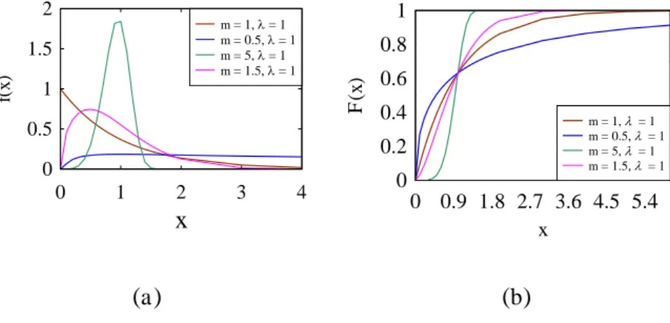
Degenerate distribution, Skellam distribution, Gamma distribution, and Weibull distribution (Figliola and Beasley, 2000). In this study, Weibull distribution is used to represent the uncertainty in the material properties. Weibull distribution has many forms. However, in this study the Weibull distribution refers to a probability distribution f(x), which is given by the following equation (Defoirdt et al., 2010; Trujillo E. , et al., 2014).
1 ) ( m x m w e x m x
f
(2.4)
Here, x [0,], m is called the form or shape parameter and is called the scale parameter. The effects of m and are shown in Figure 2.1(a).
(a) (b)
Figure 2.1:Weibull (a) density function and (b) cummulative distribution for different shape and scale factor.
The cumulative Weibull distribution takes the following form:
m
x x
w
w x f x dx e
F
( ) 1 ) (
0 (2.5)
The shape of Fw(x) is shown in Figure 2.1(b) for different values of shape and
scale parameters. The expected value and the variance of Weibull distribution are given as follows:
x
f(
x
)
0 1 2 3 4
0 0.5 1 1.5 2
m = 1, = 1 m = 0.5, = 1 m = 5, = 1 m = 1.5, = 1
x
F
(x
)
0 0.9 1.8 2.7 3.6 4.5 5.4
0 0.2 0.4 0.6 0.8 1
m = 1, = 1
m = 0.5, = 1
m = 5, = 1
33 m 1 1 (2.6) 2 2 2 2 1
m (2.7)
Here, Γ is the gamma function. Confidence interval for and σ2 at 95% confidence is calculated using Mean Time to Failure (MTTF) (Santiago; Lane, 2017; Sullivan, 2017) method.
When fw(x) is unknown but a set of data points regarding x is known, i.e., {xi | i
= 1,…,m} is known, in such case, one can apply a procedure to determine Fw(x)
first and estimate the shape and scale parameters. This way, one can determine the underlying fw(x) associated with the data points of x. There are different
types of procedures to determine Fw(x) from a set of data points (Kececioglu,
1994; Weibull, 1992-2018; Wikipidia, 2017). One of the widely used procedures, median rank approximations, is described below.
This cumulative distribution function is a step function that steps up by 1/n at each of the n data points. There are different approaches to obtaining the empirical distribution function from data. In statistics, an empirical distribution function is the distribution function associated with the empirical measure of a sample. An empirical measure is a random measure arising from a particular realization of a (usually finite) sequence of random variables. In this study, the approximation method represented by equation (2.8) is used to calculate the empirical distribution function:
4 . 0 3 . 0 ) ( n x x
F i i (2. 8)
For the step by step calculation of mean order number or empirical distribution function F (xi), (Kececioglu, 1994) xi is the rank of the data point and n is the
34
find the Weibull cumulative function for different properties and shown in Section 3.6.2.
2.2Average, Standard Deviation and Ranges of Mean and Variance
Let x(i) , i = 1,...,m, be the given data points regarding a parameter x where
m is the number of data points. The average denoted as ̅ of these data points is given by equation (2.9)
̅ =∑��= �
(2. 9)
The average provides the central tendency of the data points and is used for statistical analysis of uncertainty, as it is shown in Section 3.6.1.
The standard deviation denoted as sd of the data points, x(i) , i = 1,...,m, is given as follows:
1 ) ( 1 2
m x i x sd m i (2. 10)The standard deviation represents the dispersion in the data points and is used to quantify the uncertainty, as it is shown in Section 3.6.1.
The ranges of the expected value and variance denoted as and 2, respectively, of a given set of data points, x(i) , i = 1,...,m, are given as follows:
, 2 1 m sd t
x
(2. 11)35
In equations (2.11)(2.12), is the degree of freedom equal to m−1, is the significance level, −�⁄ ,� is the critical value of a Student's t-distribution for a two-sided test, ��⁄ ,�, and � −�⁄ ,� are the lower and upper critical values of a
2
distribution for a two-sided test. Refer to (Hiller, Lieberman, Nag, and Basu, 2005; Montgomery, 2001; Tables for Probability Distributions) for the details of the relevant distributions. Note that for a two-sided test, (1−/2)100% is the confidence interval. Usually, =0.05% or 97.5% confidence interval is used to calculate the ranges of and 2. The ranges of expected value and variance as defined above are widely used in quantifying the uncertainty associated with a given set of data points, as it is shown in Section 3.6.1.
2.3Possibility Distribution or Fuzzy Number
A fuzzy number, DoB (degree of belief) is a function DoB: [0, 1], and it must follow the following four conditions (Zadeh, 1975; Dubois and Prade, 1978; Dijkman, et al., 1983)
a) Normal,
b) Compactly supported, c) Convex, and
d) Upper semi-continuous
The function is normal means that there is, at least, one real number f0 for which DoB (f0) = 1. It is compactly supported means that the set {f | DoB(f) > 0} is bounded. It is convex means that if f1 ≤ f2 ≤ f3, then min (DoB(f1), DoB(f3)) ≤ DoB(f2) for all f1, f2, f3. It is upper semi-continuous means that the set {f | DoB(f) ≥ α} is closed for each α [0, 1]. The points corresponding to DoB(.) = 1 constitutes an interval called core. The closed interval S = [a, b] beyond which the fuzzy number DoB(.) = 0 is called support. As such, DoB(a) = 0
36
when one needs an interval or a set of intervals for a given triangular fuzzy number. In this sense, all alpha-cuts belong to the support [a, b].
To infer the most plausible value and logically consistent ranges, the truth-value of the proposition is assumed to equal to its degree of membership which gives possibility distribution. It is possible to infer the most plausible value and logically consistent ranges of TS using possibility distribution as shown in Figure 2.2.
Figure 2.2: A typical nature of fuzzy number.
In order to infer the most plausible value and logically consistent range, for example, the propositions of following form: p (Z, Y, X, Q) = Z of Y jute yarn is
XQ. Here, Z {TS}, Y {raw}, X, and Q = {MPa}. The truth-value of the proposition T (p) is equal to the fuzzy number DoB (.), i.e., T (p) = DoB(X). For example, if Z = TS, Y = raw, X = 500, and Q = MPa, then the proposition is as follows: TS of raw jute yarn is 500 MPa. The truth-value of this proposition is equal to its degree of belief as given by the possibility distribution in Figure 2.2 i.e., 0.109756098. This means that "TS of raw jute yarn is 500 MPa" is more false than true. In addition, if Z = TS, Y = jute yarn, X = 200, and Q = MPa, then the proposition is as follows: TS of raw jute yarn is 200 MPa. The truth-value of this proposition is equal to its degree of belief as given by the possibility distribution in Figure 2.2 i.e., 1. This means that "TS of raw jute yarn is 200 MPa" is true and there is no doubt about it. The above explanation implies that
TS [MPa]
D
o
B
(
T
S
)
0 400 800
0 0.2 0.4 0.6 0.8 1 1.2
TS= 200 MPa
37
the value of Z corresponding to DoB(.) = 1 is the most plausible value. The range of values of Z corresponding to DoB(Z) 0.5 is the logically consistent range of values of Z because DoB(.) 0.5 corresponds to the truth-values that is more true than false. One can also determine the expected value of Z using the centroid method (Ullah and Harib, 2006).
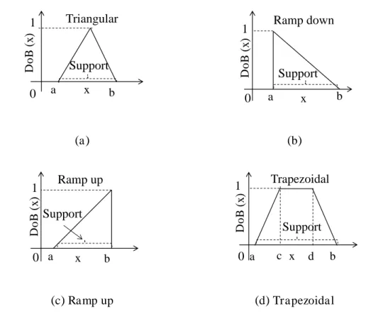
There are different categories of fuzzy numbers according to the shape of function as shown in Figure 2.3. In this study triangular Figure 2.3 (a)), ramp up (Figure 2.3 (b)), ramp down (Figure 2.3 (c)), and trapezoidal (Figure 2.3(d)) fuzzy numbers are considered. In Figure 2.3, the support of fuzzy numbers is [a, b].
(a) (b)
(c) Ramp up (d) Trapezoidal
Figure 2.3: Different shapes of the fuzzy numbers(a) triangular (b) ramp up (c) Ramp down and (d)trapezoidal.
x D o B ( x ) a b 1 0 Support Triangular x D o B ( x ) a b 1 0 Support Ramp down x D o B ( x ) a b 1 0 Support Ramp up x D o B ( x ) a b 1
0 c d
38
2.3.1 Trapezoidal Fuzzy Number
For example, Figure 2.4 shows the pictorial representation of membership function of a trapezoidal fuzzy number, DoB(x), where [b, c] is the core, [a, d] is the support, alpha cut at 50% is partially true and partially false.
Figure 2.4: Trapezoidal fuzzy number.
The following equation (2.13) represents the function of DoB (x)
otherwise d x c c x b b x a c d x c a b a x x DoB 0 1 ) ( (2. 13)
In this study trapezoidal fuzzy number is used to quantify the uncertainty of material properties, TS, as detail is shown in Chapter 3.
2.3.2 Triangular Fuzzy Number
Membership function of a triangular fuzzy number T is a fuzzy number that has a triangularly shaped membership function (DoB) expressed by equation (2.14)
b x c c x a c b x b a c a x x
T( ) (2. 14)
Core Support Alpha-cut D o B ( x ) x 1
a b c d
39
In equation (2.14), x, and a < c < b. As such, the support of the triangular fuzzy number T is [a, b]. The core of T is c because T(x = c) = 1 as shown in Figure 2.5
Figure 2.5:A triangular fuzzy number.
The function (xa)/(ca) is called the left function and the function (bx)/(bc) is called the right function. The alpha-cuts of a triangular fuzzy number are the intervals [a + (ca), b (bc)], (0, 1). Triangular fuzzy number is used to quantify the uncertainty of the physical parameter such as modulus of elasticity (E) and strain to failure (s) as shown in Chapter 3.
2.3.3 Ramp Up Fuzzy Number
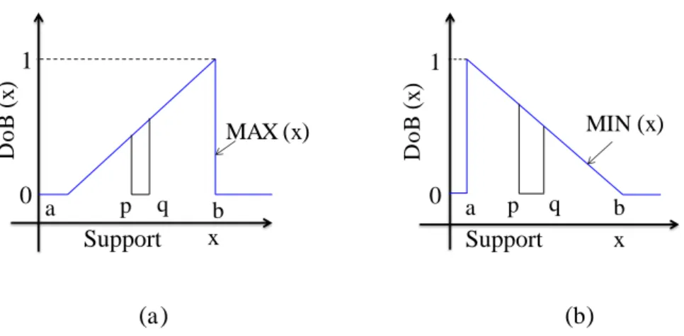
A ramp up fuzzy number denoted as MAX is also a fuzzy number. It defines a possibilistic objective function for maximizing a quantity. The expression of
MAX is given by equation (2.15):
otherwise b x a b
a x x
MAX
0
, 0 max )
( (2. 15)
The core of MAX is equal to b and the support is equal to [a, b] as shown in Figure 2.8(a). MAX linearly increases with the x in the interval of its support. Since MAX is for maximizing a quantity, it can be used as maximization function and setting its support [a, b] is a critical issue.
x
T
(
x
)
a c b
1
0
Core
40
(a) (b)
Figure 2.6: (a) Ramp up and (b) typical pattern of ramp up function.
The ramp up function is used to define the maximization function as shown in Chapter 4. In this study maximization function is used to represent the objective function of a criterion which is needed to maximize. Depending on the support the area of the MAX is changed as shown in Figure 2.6(b). This issue of support is described in Chapter 4 and 5.
2.3.4 Ramp Down Fuzzy Number
A ramp down fuzzy number denoted as MIN is also a fuzzy number as shown in Figure 2.7(a). It is defined as possibilistic objective function for minimizing a quantity. The expression of MIN is given by equation (2.16):
(a) (b)
Figure 2.7: (a) Ramp down and (b) typical pattern of ramp down function.
x
M
A
X
(
x
)
a b
1
0
Support Core
Alpha-cut
x
M
A
X
(
x
)
1
0 Support
x
M
IN
(
x
)
a b
1
0
Support Core
Alpha-cut
x
M
IN
(x
)
1
41
otherwise a x a b
x b
x MIN
0
, 0 max )
(
(2. 16)
The ramp down function is used to define the minimization function is shown in Chapter 4. The core of MIN is equal to a, and the support is equal to [a, b]. MIN
linearly decreases with the increase in x in the interval of its support. Since MIN
is for minimizing a quantity, it can be used as minimization function and setting its support [a, b] is a critical issue (see Figure 2.7(b)), similar to MAX. This issue is also described in Chapter 4. In this study minimization function is used to represent the objective function of a criterion which is needed to minimize. Application of the MIN is shown in Chapter 4 and the critical issue regarding the support selection is discussed in Chapter 5.
2.4Degree of Compliance
The interaction between the information and objective function is termed as compliance. The degree of compliance means how well the information complies with the objective functions. Its value lies between 0 and 1. When the information fully complies with the objective, the value of the compliance is 1 otherwise it is less than 1. The degree of compliance calculation is different depending on the categories of information or data. There are two broad categories of information as listed below:
a) Crisp information and
b) Granular information


![Table 3-c. Indexing of the TS , E , and s data for jute yarn. Index Number ( x i ) F (x i ) Properties TSi[MPa] Ei[GPa] s i [%] 1 0.045 33.868916 0.610077 5.03% 2 0.110 37.389838 0.624817 5.37% 3 0.175 37.458465 0.643132 5.38% 4 0](https://thumb-ap.123doks.com/thumbv2/123deta/9841399.491241/94.892.151.760.186.549/table-indexing-data-jute-index-number-properties-tsi.webp)
