Instructions for use
A uthor(s ) Nakamura,Gen; W ang,S hengzhang; W ang,Y anbo
C itation Hokkaido University Preprint S eries in Mathematics, 687: 1-26
Is s ue D ate 2005
D O I 10.14943/83838
D oc UR L http://hdl.handle.net/2115/69492
T ype bulletin (article)
F ile Information pre687.pdf
ORDER DERIVATIVE OF FUNCTIONS WITH SEVERAL VARIABLES
G. NAKAMURA, S. Z. WANG, AND Y. B. WANG†
Abstract. We propose a regularized optimization problem for computing numerical differentiation for the second order deriva-tive for functions with two variables from the noisy values of the function at scattered points, and give the proof of the existence and uniqueness of the solution of this problem. The reconstruc-tion scheme is also given during the proof, which is based on bi-harmonic Green function. The convergence estimate of the regular-ized solution to the exact solution for the regularregular-ized optimization problem as the regularized parameter and discrepancy of noisy data tending to zero is provided under a simple choice of regularization parameter. In the end we give the numerical examples and analyze the computational results.
1. Introduction
Numerical differentiation is a problem to determine the derivatives from the given noisy values of the function at scattered points. It arises from many scientific researches and applications. The differentiation of noisy data is an ill-posed problem, which means, the small errors in the measurement of the function may lead to large errors in its computed derivatives ([7], [9], [13]). There have been many methods developed ([8], [9], [12]) for treating the numerical differentiation problem. One group of methods uses Tikhonov regularization for solving the ill-posed problem([5], [7], [11]).
1991Mathematics Subject Classification. 65D25, 47A52, 34B27.
Key words and phrases. Numerical differentiation, Regularization, Green function.
†This work is partially support by NSF of China (10271032) and the Laboratory
of Nonlinear Sciences in Fudan University, Shanghai, P. R. China.
A simple but very useful solution to the problem for one variable case based on Tikhonov regularization method has been developed in ( [15], [9]). This method was used to find discontinuous solutions of Abel integral equations [3] and edge detection of image [10]. The results showed that this method was quite efficient. The higher order numer-ical differentiation by this method was given in [14]. And for the two variables case, a scheme for computing the first order derivative was given in [16] and the numerical example also showed this method was efficient. But in many applications, It is quite necessary to compute the higher order derivatives, for example, in the plate bending problem, the bending moments are obtained from the second derivatives of the primal solution [2], so in this paper we will give the solution for two variables case. For the cases of the number of variables more than two, the same argument given in this paper still works.
The paper is organized as follows: in section 2, we discribe the prob-lem in detail and prove the existence and uniqueness of the solution; in section 3 we prove the convergence of our method by error estimate; the numerical examples are given in section 4 and we conclude this method in terms of the results of the numerical examples in section 5; we give the algorithm for computing the Green function in Appendix.
2. Problem and some results
Suppose that Ω ⊂ R2 is a simply connected bounded domain and
̺ = ̺(x) is a function defined in Ω. Let N be a natural number and
{xi}Ni=1 be a group of points in Ω. We assume that Ω is divided into
N parts {Ωi}Ni=1, and there is only one point of {xi}Ni=1 in each part.
For simplicity we also assume that the volumes of all Ωi are same. We
denote di as the diameter of Ωi and let d= max{di}.
We will discuss the following problem:
Suppose that we know the approximate value ˜̺i of ̺(x) at point xi,
i.e.
(2.1) |̺˜i−̺(xi)| ≤δ, i= 1,2,· · · , N,
We want to find a function f∗(x) approximates function ̺(x) such
that kf∗−̺kH2(Ω) is small and
lim
h→0,δ→0kf∗−̺kH
2
(Ω)= 0.
Assuming that there are two functions φ(x)∈H7/2(∂Ω) and ϕ(x)∈
H3/2(∂Ω) satisfyingkφ(x)−̺(x)k
H7/2(∂Ω) ≤δandkϕ(x)−△̺(x)kH3/2(∂Ω) ≤
δ, we treat this problem as the following optimization problem by using
Tikhonov regularization method.
Problem 2.1. Define a cost functional Φ(f):
Φ(f) = 1
N N X
j=1
(f(xj)−̺˜j)2+αk△2fk2L2
(Ω), f ∈H
where H = {f|f ∈ H4(Ω), f|∂Ω = φ,△f|∂Ω = ϕ}, and α > 0 is a
regularization parameter.
The problem is then to find f∗ ∈H such that Φ(f∗)≤Φ(f)for every f ∈H.
Then we will prove the existence and uniqueness of the minimizer of Problem 2.1.
Theorem 2.2. Suppose that f∗ ∈ H is the solution of the following
variational problem:
(2.2)
Z
Ω
△2f△2hdx=− 1
αN N X
j=1
(f(xj)−̺˜j)h(xj)
for all h ∈ Hˆ = {h|h ∈ H4(Ω), h|∂Ω = △h|∂Ω = 0}. Then f∗ is the
minimizer of Problem 2.1. Moreover, the minimizer of Problem 2.1 is unique.
Remark 2.3. We will prove the existence of a solution of (2.2) later
Proof of Theorem 2.2: For anyf ∈H, leth=f−f∗, thenh|∂Ω= 0
and △h|∂Ω= 0. It is easy to have the following equations:
Φ(f)−Φ(f∗) =
1
N N X
j=1
(f(xj)−f∗(xj))(f(xj) +f∗(xj)−2˜̺j)
+α
Z
Ω
£
(△2f)2−(△2f∗)2
¤
dx
(2.3)
= I1 +αI2
and
I1 =
1
N N X
j=1
h(xj)(2f∗(xj)−2 ˜̺j +h(xj))
= 1
N N X
j=1
2(f∗(xj)−̺˜j)h(xj) +h2(xj).
By the definition of f∗, we have
I2 =
Z
Ω
[(△2f)2−(△2f∗)2]dx=k△2hk2L2
(Ω)+ 2
Z
Ω
△2h· △2f∗dx
= k△2hk2L2(Ω)−
2
αN N X
j=1
(f∗(xj)−̺˜j)h(xj).
Substituting the equations I1 and I2 into (2.3) gives
Φ(f)−Φ(f∗) = 1
N N X
j=1
h2(xj) +αk△2f − △2f∗k2L2(Ω)≥0.
Thus, f∗ is a minimizer of Problem 2.1.
If there is anotherf∗ ∈H minimizing Problem 2.1, denoteg =f∗−
f∗, then functiong satisfies:
R
Ω(△2g)2dx= 0 andg|∂Ω = 0,△g|∂Ω = 0.
Hence, g(x)≡ 0 for x ∈ Ω. So f∗ = f
∗. Therefore, the uniqueness of
the minimizer of Problem 2.1 has been proven. ¤
To completely solve numerical differentiation problem, it is
neces-sary to provide a scheme for constructing f∗. For that, by an a priori
f∗. A theorem will also be given to prove that the constructedf∗ is the
solution of (2.2).
Let’s recall the definition of a bi-harmonic Green function before the
construction. FunctionG(x, y) with fixedy∈Ω is called a bi-harmonic
Green function if it satisfies the following equations:
△2xG(x, y) =δ(x−y) in Ω
and
G|∂Ω = 0,△xG|∂Ω = 0.
We can obtain G(x, y) by solving
△xF(x, y) =δ(x−y) in Ω
F(x, y)|∂Ω = 0
and
△xG(x, y) =F(x, y) in Ω
G(x, y)|∂Ω = 0.
We denote△1 as the Laplacian operator for the first argument, and△2
as the Laplacian operator for the second argument. Since G(x, y) =
G(y, x) andF(x, y) = F(y, x) for x, y ∈Ω, then we will have
(2.4) △2G(y, x) =△1G(x, y) =F(x, y) =F(y, x) =△1G(y, x).
Now we will propose a scheme to obtain the solution of the Eq. (2.2).
Takingh=G(x, y) in (2.2) and using the definition of Green function,
we obtain
−1
N N X
j=1
(f∗(xj)−̺˜j)G(xj, y) =
Z
Ω
α△2f∗(x)· △2xG(x, y)dx
= α△2f
Multiply two sides of the above equation with G(x, y) and integrate it on Ω, we obtain by integrating by parts
−1
N N X
j=1
(f∗(xj)−̺˜j)
Z
Ω
G(xj, x)G(x, y)dx
= α
Z
Ω
△2f∗(x)·G(x, y)dx
= α
Z
∂Ω
( ∂
∂ν△f∗(x)·G(x, y)− ∂
∂νG(x, y)· △f∗(x))ds(x)
+α
Z
Ω
△f∗(x)· △xG(x, y)dx
= −α
Z
∂Ω
∂
∂νG(x, y)·ϕ(x)ds(x)−α
Z
∂Ω
∂
∂ν△xG(x, y)·φ(x)ds(x)
+αf∗(y),
where ν is the unit normal of ∂Ω directed outside Ω. Rewrite the
above equation in the form:
αf∗(x) +
1
N N X
j=1
(f∗(xj)−̺˜j)
Z
Ω
G(xj, y)G(y, x)dy
(2.5)
= α
Z
∂Ω
∂
∂νG(y, x)·ϕ(y)ds(y) +α
Z
∂Ω
∂
∂ν△yG(y, x)·φ(y)ds(y).
By defining
(2.6) aj(x) =
Z
Ω
G(xj, y)G(y, x)dy,
(2.7)
b(x) =
Z
∂Ω
∂
∂ν△yG(y, x)·φ(y)ds(y) +
Z
∂Ω
∂
∂νG(y, x)·ϕ(y)ds(y),
and
(2.8) cj =−
1
αN(f∗(xj)−̺˜j)
then (2.5) becomes
(2.9) f∗(x) =
N X
j=1
Now the problem of constructing f∗ reduces to computing the
coef-ficients cj from ˜yj ϕ(x) and φ(x). From (2.8) and (2.9) we obtain
(2.10) cj =−
1
αN(f∗(xj)−̺˜j) = −
1
αN( N X
k=1
ak(xj)ck+b(xj)−̺˜j).
Let
A=
αN +a1(x1) a2(x1) a3(x1) · · · aN(x1)
a1(x2) αN +a2(x2) a3(x2) · · · aN(x2)
· · · ·
a1(xN) a2(xN) a3(xN) · · · αN +aN(xN)
and
c=
c1
c2
· · ·
cN
,b=
˜
y1−b(x1)
˜
y2−b(x2)
· · ·
˜
yN −b(xN).
,
Then (2.10) becomes the linear equations Ac = b. Solving this
equations, we will obtain coefficientscj, which finishes the construction
of f∗.
Theorem 2.4. Suppose functionf∗ =PN
j=1cjaj(x) +b(x) whereaj(x)
andb(x) are defined in (2.5)and (2.6),{cj}Nj=1 is the solution of linear
system (2.10), then f∗ is the solution of (2.2).
Proof. For every x ∈ ∂Ω, from the definition of Green function, we
know that G(x, y) = G(y, x) = 0 fory ∈Ω. So
aj(x) = Z
Ω
G(xj, y)·G(y, x)dy = 0.
Assume that ˆφ∈H2(Ω) is an extension ofφ to Ω and ˆϕ ∈H2(Ω) is an
extension of ϕ over Ω, then integrating by parts yields
b(x) = φ(x) (x∈∂Ω).
Thus we have f∗(x)|∂Ω=φ(x).
We also have
△aj(x) = Z
Ω
Since
b(x) =
Z
Ω
ˆ
φ(y)△2yG(y, x)dy− Z
Ω
△yG(y, x)△φˆ(y)dy
+
Z
Ω
ˆ
ϕ(y)△yG(y, x)dy− Z
Ω
G(y, x)△ϕˆ(y)dy (x∈∂Ω),
then we will have using the definition ofF(x, y) and (2.4),
△b(x) = △φˆ(x)− Z
Ω
△x(△yG(y, x))△φˆ(y)dy
+
Z
Ω
ˆ
ϕ(y)△x(△yG(y, x))dy− Z
Ω
△xG(x, y)△ϕˆ(y)dy
= △φˆ(x)−
Z
Ω
△2xG(x, y)△φˆ(y)dy+
Z
Ω
ˆ
ϕ(y)△2xG(x, y))dy
= ϕ(x) (x∈∂Ω).
Thus we have △f∗(x)|∂Ω=ϕ(x).
Moreover, from the definition of aj(x) and b(x), we know that for
every x∈Ω
(2.11) △2aj(x) =
Z
Ω
G(xj, y)△2xG(x, y)dy =G(xj, x)
and (2.12)
△2b(x) = △ϕˆ(x)− Z
Ω
△2xG(x, y)△ϕˆ(y)dy =△ϕˆ(x)− △ϕˆ(x) = 0.
Since G(xj, x) ∈ L2(Ω) , so △2f∗(x) ∈ L2(Ω). By the priori estimate
of Poisson equation with Dirichlet boundary condition (see Lemma 3.2
For any h∈Hˆ, we have
Z
Ω
△2f∗△2hdx =
Z
Ω
N X
j=1
cjG(xj, x)△2h(x)dx
=
N X
j=1
cj µZ
Ω
△G(xj, x)△h(x)dx− Z
∂Ω
△h(x)∂G(xj, x)
∂ν ds(x)
+
Z
∂Ω
G(xj, x)
∂△h(x)
∂ν ds(x)
¶
=
N X
j=1
cj µZ
Ω
△2G(xj, x)h(x)dx− Z
∂Ω
h(x)∂△G(xj, x)
∂ν ds(x)
+
Z
∂Ω
△G(xj, x) ∂h(x)
∂ν ds(x)
¶
=
N X
j=1
cjh(xj) = −
1
αN N X
j=1
(f∗(xj)−̺˜j)h(xj).
Sof∗ is the solution of (2.2). This completes the proof. ¤
The solution of the linear equations exists and is unique since if we
assume ˜yi = 0, i= 1,· · · , N, and φ(x) =ϕ(x) = 0, then we know that
there is only one minimizer of Problem 2.1 , which isf∗(x)≡0, x∈Ω.
It is obvious c = 0 is a solution of Ac = 0 and if there is another ˆc
satisfying Aˆc= 0, then we will have a function ˆf 6= 0 which is also a
minimizer of Problem 2.1. This is a contradiction so the homogenous linear equations only has a trivial solution. Thus the solution of the linear equations exists and is unique.
3. Error estimate
In this section we will prove a convergence estimate for our proposed solution under a priori choice of the regularization parameter. The proof uses the following two Lemmas.
Lemma 3.1. LetΩbe a domain inRn having the strong local Lipschitz
property, u∈W1,p(Ω), and suppose that n < p≤ ∞ , then
|u(x)−u(y)| ≤K|x−y|1−npkuk 1,p,Ω
This lemma can be obtained from Lemma 5.17 in page 108 of [1].
Lemma 3.2. LetΩbe aC1,1 domain in Rn, and let the operatorLu=
aij(x)D
iju+bi(x)Diu+c(x)u be strictly elliptic in Ω with coefficients aij ∈ C0(Ω), bi, c ∈ L∞, with i, j = 1,· · · , n and c ≤ 0. Then there
exists a constant C (independent of u) such that
kuk2,p,Ω ≤CkLukp,Ω
for all u∈W2,p(Ω)∩W01,p(Ω),1< p <∞.
This lemma can be obtained from Lemma 9.17 in page 242 of [6]. According to the result of [4], we choose the regularization parameter
α = δ2. Such choice has been proven to be quite effective (see [15]).
We give the error estimate in the following theorem:
Theorem 3.3. Suppose Ω satisfies the conditions in Lemma 3.1 and
Lemma 3.2, and f∗ is the minimizer of Problem 2.1 and y ∈ H4(Ω).
Let e = f∗ −y and choose α = δ2, then we have the following error
estimate
k△ekL2 ≤L1d 1 2 +L
2δ
1
2, kek
L2 ≤L3d+L4δ
k∇ekL2 ≤L
5d
3 4 +L
6δ
1
2, k∇△ek
L2 ≤L
7d
1
4 +L
8δ
1 4
where Li are constants which depend on Ω, kφkH7/2(∂Ω), kϕkH3/2(∂Ω) and k△2yk
L2.
Proof. First since δ2k△2f
∗k2L2 ≤ Φ(f∗) ≤ Φ(y) ≤ δ2 +δ2k△2yk2
L2, it
is easy to see that k△2ek
L2 ≤ 1 + 2k△2ykL2. Also, from the
well-posedness of the boundary value problem :
(3.1)
(
△2e=g in Ω
e=k, △e=ℓ on ∂Ω
with given g ∈ L2(Ω), k ∈ H7/2(∂Ω), ℓ ∈ H3/2(∂Ω) and the
conti-nuity of the trace operator, there are constants C1 and C2 such that
k∂
∂νekL2(∂Ω) ≤ C1 and k ∂
∂ν△ekL2(∂Ω) ≤ C2. Hereafter, Ci’s are
gen-eral constants which may depend on Ω, kφkH7/2
(∂Ω), kϕkH3/2
(∂Ω) and
k△2yk
So, by kekL2(∂Ω) ≤δ, k△ekL2(∂Ω) ≤δ,
k△ek2L2 =
Z
Ω
|△e|2dx
=
Z
∂Ω
△e· ∂
∂νedS−
Z
∂Ω
e· ∂
∂ν△edS+
Z
Ω
△2e·edx
≤ kekL2 · k△2ekL2 +C1δ+C2δ.
Here, note that the general constants C1, C2 can be different in each
estimate. We rewrite kekL2 as
kek2
L2 =
Z
Ω
e2(x)dx=
N X
i=1
Z
Ωi
e2(x)dx
=
N X
i=1
Z
Ωi
e(x)(e(x)−e(xi))dx+ N X
i=1
Z
Ωi
e(xi)(e(x)−e(xi))dx
+
N X
i=1
Z
Ωi
e2(xi)dx
= I3 +I4+I5.
Now we estimate I3, I4, and I5.
I3 =
N X
i=1
Z
Ωi
e(x)(e(x)−e(xi))dx≤ N X
i=1
Z
Ωi
|e(x)||(e(x)−e(xi))|dx
≤ N X
i=1
Z
Ωi
C1|x−xi|1− n pkek
1,p|e(x)|dx≤d1− n pC
1kek1,p Z
Ω
|e(x)|dx
≤ d1−npC
1kek1,pkekL2(vol(Ω)) 1 2
where vol(Ω) is the volume of Ω. The second inequality is obtained
from Lemma 3.1 with n = 2. We may setp= 4, then
I3 ≤d
1 2C
1(vol(Ω))
1 2kek
1,4kekL2.
From the imbedding theorem of Soblev spaces we know thatW2,2(Ω)→
W1,4(Ω) for Ω having cone property, which means, there is a constant
C1independent ofesatisfyingkek1,4 ≤C1kek2,2. By the well-posedness
of (3.1)
kek2,2 ≤C1k△ekL2 +C
Hence, we have I3 ≤C1d
1 2kek
L2(k△ek
L2 +δ).
By the same way, we have
I4 =
N X
i=1
Z
Ωi
e(xi)(e(x)−e(xi))dx≤ N X
i=1
Z
Ωi
|e(xi)||(e(x)−e(xi))|dx
≤ d12C
1kek1,4
N X i=1 ( Z Ωi
|e(xi)|dx) =d
1 2C
1kek1,4
vol(Ω)
N N X
i=1
|e(xi)|.
And since Φ(f∗)≤Φ(y), we have
1
N N X
i=1
(f∗(xi)−̺˜i)2 ≤δ2(1 +k△2̺k2).
So 1 N N X i=1
|e(xi)| ≤
1
N N X
i=1
(|f∗(xi)−̺˜i|+|̺˜i−̺(xi)|)
≤ v u u t1 N N X i=1
|f∗(xi)−̺˜i|2+δ
≤ δ(p1 +k△2̺k2+ 1).
Hence, we have I4 ≤C1d
1
2δ(k△ek+δ).
The estimation of I5 is simple
I5 =
N X
i=1
Z
Ωi
e2(xi)dx= N X
i=1
e2(xi) Z
Ωi
dx≤ 1
Nvol(Ω)· N X
i=1
e2(xi)
≤ 2
Nvol(Ω)· N X
i=1
((f∗(xi)−̺˜i)2+ ( ˜̺i−̺(xi))2)
≤ 2vol(Ω)δ2(2 +k△2̺k2) = C1δ2.
From all above, we can conclude that
kek2L2 ≤C1d 1 2kek
L2(k△ek
L2 +δ) +C2d 1
2δk△ek
L2 +C3δ2.
Then we will have
kekL2 ≤ C1d 1
2(k△ek
L2 +δ) +C2d 1 4δ
1 2k△ek
L2 +C3δ
≤ C1d
1 2k△ek
L2 +C
So it comes out the results of the theorem:
k△ekL2 ≤C1d 1
2 +C
2δ
1 2
and
kekL2 ≤C1d+C2δ
Also, since
k∇ek2L2 =
Z
Ω
∇e· ∇edx
= −
Z
Ω
△e·edx+
Z
∂Ω
e· ∂
∂νedS
≤ kekL2 · k△ekL2 +C1δ.
k∇△ek2L2 =
Z
Ω
∇△e· ∇△edx
= −
Z
Ω
△2e· △edx+
Z
∂Ω
△e· ∂
∂ν△edS
≤ k△ekL2 · k△2ekL2 +C1δ.
then we will have
k∇ekL2 ≤C1d 3
4 +C
2δ
1 2
k∇△ekL2 ≤C
1d
1
4 +C
2δ
1 4 .
This completes the proof. ¤
Remark 3.4. In this paper, for the simplicity, we assume that the
volumes of all Ωi are same. In the real application, this condition may
be not easy to be satisfied. But if we denote V1 = maxi{vol(Ωi)} and
V2 = mini{vol(Ωi)} and let VV12 is bounded with some constant, then
we still have the same error estimate.
Remark 3.5. In Theorem 3.3, we used Lemma 3.1 to estimate I3 in
which we choose the parameter p to be 4. Actually we can choose any
p satisfying2≤p <∞. And we can still use the imbedding theorem of Soblev spaces W2,2(Ω)→W1,p(Ω). The result will be
k△ekL2 ≤L1p·d1− 2
p +L
2pδ
1
2, kek
L2 ≤L3pd2− 4
p +L 4pδ
k∇ekL2 ≤L
5pd
3 2−
3
p +L
6pδ
1
2, k∇△ek
L2 ≤L
7pd
1 2−
1
p +L
8pδ
where Lip are constants depending on kφkH7
2(∂Ω), kϕkH 3
2(∂Ω) and Ω,
k△2yk
L2 and p. So when we choose a larger p we will get a better
convergence rate.
4. Numerical examples
We provide numerical examples in this section.
For constructing f∗ and △f∗, we compute the Green function G by
Fourier series and denote the number of terms in Fourier series by K.
We give the detailed algorithm of the construction in Appendix.
We compute△f∗ from ˜̺i (1≤i≤N) satisfying (2.1) with
̺(x, y) = (2−(2x−1)2)2sin (ay)
wherea is a constant. We setδ = 0.001, divide Ω intoN parts {Ωi}N1 .
We evaluate the computed relative error by the formulae
e1 =
³ PN
j=1(f∗(xj)−̺(xj))2
´1/2
³ PN
i=1(̺(xj))2
´1/2 ,
e2 =
³ PN
j=1(△f∗(xj)− △̺(xj))2 ´1/2
³ PN
i=1(△̺(xj))2
´1/2 .
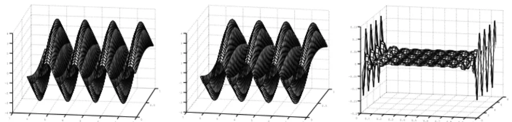
First, we set a = 4 in function ̺(x, y), and choose N = 402 and
K = 100, then Fig. 1 and Fig. 2 show our numerical results. In Fig.
1, the left figure shows exact value of ̺(x, y), the middle one shows
the constructed functionf∗(x, y), and the right one shows difference of
f∗(x, y) and ̺(x, y) which is f∗ −̺. In Fig. 2, the left figure shows
exact value of △̺(x, y), the middle one shows constructed function
△f∗(x, y), and the right one shows the difference△f∗− △̺.
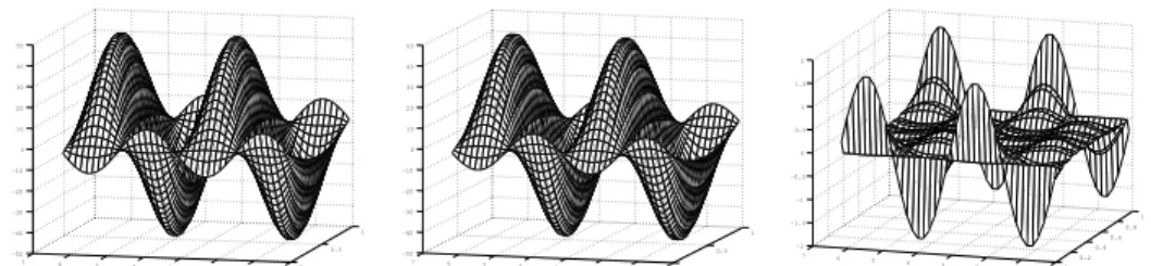
Fig. 3 and Fig. 4 show our numerical results when a = 2. Fig.
3 is about constructed f∗ and Fig. 4 is about △f∗, and each figure
corresponds to the same item as in Fig. 1 and in Fig. 2.
Fig. 5 and Fig. 6 show our numerical results when a = 0.5. Fig.
3 is about constructed f∗ and Fig. 4 is about △f∗, and each figure
0 0.5 1 0 1 2 3 4 5 6 7 -4 -3 -2 -1 0 1 2 3 4 0 0.5 1 0 1 2 3 4 5 6 7 -4 -3 -2 -1 0 1 2 3 4
0 0.1 0.2 0.3 0.4 0.5 0.6 0.7 0.8 0.9 1 0 2 4 6 8 -0.2 -0.15 -0.1 -0.05 0 0.05 0.1 0.15
Figure 1. The left figure shows exact value of ̺(x, y)
whena= 4, the middle figure shows constructed function
f∗(x, y), and the right figure shows the difference f∗ −̺
0 0.5 1 0 1 2 3 4 5 6 7 -100 -80 -60 -40 -20 0 20 40 60 80 100 0 0.5 1 0 1 2 3 4 5 6 7 -100 -80 -60 -40 -20 0 20 40 60 80 100 0 0.5 1 0 1 2 3 4 5 6 7 -0.2 -0.15 -0.1 -0.05 0 0.05 0.1 0.15 0.2
Figure 2. The left figure shows exact value of ∆̺(x, y)
whena= 4, the middle figure shows constructed function
∆f∗(x, y), and the right figure shows the difference△f∗−
△̺ 0 0.5 1 0 1 2 3 4 5 6 7 -4 -3 -2 -1 0 1 2 3 4 0 0.5 1 0 1 2 3 4 5 6 7 -4 -3 -2 -1 0 1 2 3 4 0 0.2 0.4 0.6 0.8 1 0 1 2 3 4 5 6 7 -0.2 -0.15 -0.1 -0.05 0 0.05 0.1 0.15
Figure 3. The left figure shows exact value of ̺(x, y)
whena= 2, the middle figure shows constructed function
f∗(x, y), and the right figure shows the difference f∗ −̺
In all the right figures, we can find the errors near the boundary of the domain Ω are much larger than the errors inside. Therefore, we
define Ω′ which equals Ω minus a band near the boundary with widthε
and compute the relative errorse1 ande2 only in Ω′. We always choose
0 0.5 1 0 1 2 3 4 5 6 7 -50 -40 -30 -20 -10 0 10 20 30 40 50 0 0.5 1 0 1 2 3 4 5 6 7 -50 -40 -30 -20 -10 0 10 20 30 40 50 0 0.2 0.4 0.6 0.8 1 0 1 2 3 4 5 6 7 -2 -1.5 -1 -0.5 0 0.5 1 1.5 2
Figure 4. The left figure shows exact value of ∆̺(x, y)
whena= 2, the middle figure shows constructed function
∆f∗(x, y), and the right figure shows the difference△f∗−
△̺ 0 0.5 1 0 1 2 3 4 5 6 7 0 0.5 1 1.5 2 2.5 3 3.5 4 0 0.5 1 0 1 2 3 4 5 6 7 0 0.5 1 1.5 2 2.5 3 3.5 4 0 0.2 0.4 0.6 0.8 1 0 1 2 3 4 5 6 7 -0.14 -0.12 -0.1 -0.08 -0.06 -0.04 -0.02 0 0.02 0.04
Figure 5. The left figure shows exact value of ̺(x, y)
whena = 0.5, the middle figure shows constructed
func-tion f∗(x, y), and the right figure shows the difference
f∗ −̺
0 0.2 0.4 0.6
0.8 1 0 2 4 6 8 -35 -30 -25 -20 -15 -10 -5 0 5 10 15 0
0.2 0.4 0.6
0.8 1 0 2 4 6 8 -40 -30 -20 -10 0 10 20 0 0.5 1 0 1 2 3 4 5 6 7 -2.5 -2 -1.5 -1 -0.5 0 0.5
Figure 6. The left figure shows exact value of ∆̺(x, y)
whena = 0.5, the middle figure shows constructed
func-tion ∆f∗(x, y), and the right figure shows the difference
△f∗− △̺
We also investigate the errors with K and N being changed.
Table 1. Relative errors(%) of constructedf∗ and△f∗
for different a in functions ̺(x, y) and △̺(x, y) (N =
402, K = 100), respectively
a 4 2 0.5
e1 0.2794 0.2279 0.2312
e2 0.1114 0.6175 1.3245
Table 2. Relative errors of f∗ and △f∗ with different
K’s(%)(fix N = 402)
K = 80 K = 100 K = 120
e1 0.2908 0.2794 0.1815
a=4
e2 1.3034 0.1114 0.1114
e1 0.2144 0.2279 0.0846
a=2
e2 3.1704 0.6175 0.5595
e1 0.2122 0.2312 0.0927
a=0.5
e2 4.9742 1.3245 1.2260
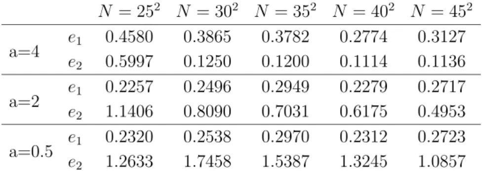
Table 3. Relative errors of f∗ and △f∗ with different
N’s(%)(fixK = 100)
N = 252 N = 302 N = 352 N = 402 N = 452
e1 0.4580 0.3865 0.3782 0.2774 0.3127
a=4
e2 0.5997 0.1250 0.1200 0.1114 0.1136
e1 0.2257 0.2496 0.2949 0.2279 0.2717
a=2
e2 1.1406 0.8090 0.7031 0.6175 0.4953
e1 0.2320 0.2538 0.2970 0.2312 0.2723
a=0.5
e2 1.2633 1.7458 1.5387 1.3245 1.0857
We choose N = M2 and increase M from 25 to 45 with increment
equal 5 in each time. Table 3 gives the computed results of relative errors.
5. Discussion and conclusion
In the numerical examples, we can see when we choose K = 100
andN = 402, the constructedf
functions̺(x, y) and△̺(x, y) with different a’s in Fig. 1 - Fig 6. From
Table 1, we can see that forf∗ the relative errorse1’s are less than 0.3%,
and for △f∗ the relative errore2 increases from 0.1114% to 1.3245%.
In Table 2, we can see that when increasing K from 80 to 120, both
e1 ande2 decrease. So increasing the number of terms in Fourier series
can improve the numerical results of our method.
In Table 3, we can see that when incresing N from 252 to 452, e
1’s
have small oscillation and the values are less than 0.5% for three cases.
bute2’s change are a little bit complicated. Fora = 4 case,e2 decreases
from 0.5997% to 0.1136%. For a = 2 case, e2 decreases from 1.1406%
to 0.4953%. For a = 0.5 case, e2 decreases from 1.2633 to 1.0857. So
by increasing N, we can improve the numerical results very much for
a= 4, but the improvement is a little fora = 0.5. This fact tells us that
increasing N for the domain decomposition {Ω}N
i=1 can also improve
the numerical results of our numerical differentiation for the second derivative of functions with two variables, but the error depends on the property of the original function. As shown in Appendix B, we use sine series to compute the Green function, but computing in this way is not very accurate if the original function is not an odd function. Also for non-odd functions, we can observe that by using sine series, the result is better for rapidly oscillating functions than slowly oscillating functions. Due to the memory limitation problem of our computer, we
could not take a larger N for the domain decomposition and a larger
K which bounds (k1, k2) such that 1≤k1, k2 ≤K for the Fourier series
to make our numerical results precise enough. We expect that if we
can take N, K larger, we can make our results more precise.
References
[1] Adams, R. A.: Sobolev Spaces. Pure and Applied Mathematics, Vol. 65, Aca-demic Press, New York-London, 1975.
[2] Brezzi, F., Fortin, M.: Mixed and Hybrid Finite Element Methods. Springer Series in Computational Mathematics, Vol. 15, Springer-Verlag, New York 1991.
[4] Cheng, J., Yamamoto, M.: One new strategy for a priori choice of regularizing parameters in Tikhonov’s regularization. Inverse Problems 16 (2000), pp. 31-38.
[5] Engl, H. W., Hanke, M., Neubauer, A.: Regularization of Inverse Problems. Kluwer Academic Publishers, Dordrecht Hardbound, 1996.
[6] Gilbarg, D., Trudinger, N. S.: Elliptic Partial Differential Equations of Second Order. Springer-Verlag Berlin Heidelberg, 2001.
[7] Groetsch, C. W.: The Theory of Tikhonov Regularization for Fredholm Equa-tions of the First Kind. Research Notes in Mathematics, 105. Pitman (Ad-vanced Publishing Program), Boston, Mass.-London 1984.
[8] Groetsch, C. W.: Differentiation of approximately specified functions. Amer. Math. Monthly 98 (1991), pp. 847-850.
[9] Hanke, M., Scherzer, O.: Inverse problems light: numerical differentiation. Amer. Math. Monthly 108 (2001), no. 6, pp. 512-521.
[10] Hon, Y. C., Wang, Y. B., Cheng, J.: A Numerical differentiation method for edge detection. Preprint City University of Hong Kong, Hong Kong 2003. [11] Murio, D. A.: The Mollification Method and the Numerical Solution of
Ill-posed Problems. A Wiley-Interscience Publication. John Wiley & Sons, Inc., New York, 1993.
[12] Ramm, A. G., Smirnova, A. B.: On stable numerical differentiation. Math. Comp. 70 (2001), pp. 1131-1153.
[13] Tikhonov, A. N., Arsenin, V. Y.: Solutions of Ill-posed Problems. Winston and Sons, Washington, 1977.
[14] Wang, Y. B., Hon, Y. C., Cheng, J.: Reconstruction of High Order Derivatives from Input Data. Submitted to Journal of Inverse and Ill-posed Problems, (2004).
[15] Wang, Y. B., Jia, X. Z., Cheng, J.: A numerical differentiation method and its application to reconstruction of discontinuity. Inverse Problems 18 (2002), pp. 1461-1476.
6. Appendix A: Proof of G(x, y) = G(y, x)
Here we will give the proof that the solutionG(x, y) with fixedy∈Ω
of
△2xG(x, y) =δ(x−y) in Ω
G(x, y)|∂Ω =△xG(x, y)|∂Ω = 0
satisfies G(x, y) = G(y, x), for any x, y ∈Ω.
Proof: Supposex, yare two points in Ω. We defineBδ(x) = z||z−x|< δ, z ∈Ω,
Bδ(y) = {z||z − y| < δ, z ∈ Ω}, and Ωδ = Ω \ (Bδ(x)∪Bδ(y)),
Γδ(x) = ∂Bδ(x), Γδ(y) = ∂Bδ(y). According to Green formula, we
know that for any u, v ∈H4
Z
Ωδ
△2xu·v dx =
Z
∂Ωδ ∂ ∂νx
△xu·v ds− Z
∂Ωδ
△xu· ∂ ∂νx
v ds
+
Z
∂Ωδ ∂ ∂νx
u· △xv ds
− Z
∂Ωδ u· ∂
∂νx
△xv ds+ Z
Ωδ
u· △2xv dx
So
Z
Ωδ
△2zG(z, x)·G(z, y)dz =
Z
∂Ωδ ∂ ∂νz
△zG(z, x)·G(z, y)ds
− Z
∂Ωδ
△zG(z, x)· ∂ ∂νz
G(z, y)ds+
Z
∂Ωδ ∂ ∂νz
G(z, x)· △zG(z, y)ds
− Z
∂Ωδ
G(z, x)· ∂
∂νz
△zG(z, y)ds+ Z
Ωδ
G(z, x)· △2
zG(z, y)dz
=I1(δ)−I2(δ) +I3(δ)−I4(δ) +
Z
Ωδ
G(z, x)· △2zG(z, y)dz
Since y, x6∈Ωδ, so for any z ∈Ωδ with z =6 x, z6=y, △2zG(z, y) = 0,
△2
zG(z, x) = 0.
Hence we have
I1(δ)−I2(δ) +I3(δ)−I4(δ) = 0
Next we will prove that limδ→0I2(δ) = 0,limδ→0I3(δ) = 0, and
LetF(z, x) =△zG(z, x), then
△zF(z, x) =δ(z−x) in Ω
F(z, x)|∂Ω = 0
SoF(z, x)∈C∞ for z ∈Ω\ {x}, and F(z, x)∼ 21πln|z−x|,(z →x).
Since G(z, x) = G(z, y) = △zG(z, x) = △zG(z, y) = 0(z ∈∂Ω)
I2(δ) =
Z
Γδ(x)
+
Z
Γδ(y) .
Here
Z
Γδ(x)
∼ 1
2π
Z
Γδ(x)
ln|z−x| ∂
∂νz
G(z, y)dz = 1
2π
Z 2π
0
(δlnδ) ∂
∂νG(δ, θ)
and∂ν∂zG(z, y) is bounded, soR
Γδ(x)→0 when δ→0.
As for R
Γδ(y),
Z
Γδ(y)
F(z, x) ∂
∂νz
G(z, y)ds = F(y, x)
Z
Γδ(y) ∂ ∂νz
G(z, y)ds
+
Z
Γδ(y)
(F(z, x)−F(y, x)) ∂
∂νz
G(z, y)ds.
Here,
Z
Γδ(y) ∂ ∂νz
G(z, y) =
Z
Bδ(y)
F(z, y)∼ 1
2π
Z 2π
0
dθ
Z δ
0
rlnrdθ →0
Since△zG(z, y) = F(z, y)∼ 21π ln|z−y| ∈L2 neary, by the interior
regularity for the Poison equation, we have G(z, y) ∈ H2 near y and
hence ∂
∂νzG(z, y)∈H
1
2 neary. So
Z
Γδ(y)
(F(z, x)−F(y, x) ∂
∂νz
G(z, y)→0, as δ→0
thus we have
I2(δ)→0, as δ →0
By using the same way , we will have
I3(δ)→0, as δ →0
I1(δ) =
Z
∂Ωδ ∂ ∂νz
F(z, x)G(z, y)ds = (
Z
Γδ(x)
+
Z
Γδ(y)
) ∂
∂νz
F(z, x)G(z, y)ds
We know that F(z, x)∈C∞ near y, and G(z, y)∈H2 which means
G(z, y)∈C1−ǫ. So we have
Z
Γδ(y) ∂ ∂νz
F(z, x)G(z, y)ds→0(δ→0).
As for R
)Γδ(x),
Z
Γδ(x) ∂ ∂νz
F(z, x)G(z, y) = G(x, y)
Z
Γδ(x) ∂ ∂νz
F(z, x)
+
Z
Γδ(x)
(G(z, y)−G(x, y)) ∂
∂νz
F(z, x).
Since F(z, x)∼ 21πln|z−x|, ∂ν∂zF(z, x)∼ 2π|z1−x|, G(z, y)−G(x, y) =
O(|z−x|) for z near x,
Z
Γδ(x)
(G(z, y)−G(x, y)) ∂
∂νz
F(z, x)ds →0(δ→0)
and
Z
Γδ(x) ∂ ∂νz
F(z, x)ds∼ 1
2π
Z 2∗π
0
δδ−1dθ = 1(δ→0).
ThusI1(δ)→G(x, y) as δ →0.
By the same way, we can prove thatI4(δ)→G(y, x), asδ→0. This
7. Appendix B: Algorithm of computing G(x, y) and △f∗(x)
Assume Ω = (0, L)×(0,2π) and fix y∈Ω. The problem of solving
△2xG(x, y) =δ(x−y) in Ω
G(x, y)|∂Ω =△xG(x, y)|∂Ω = 0
can be changed into solving
△xF(x, y) = δ(x−y) in Ω
F(x, y)|∂Ω = 0
and
△xG(x, y) =F(x−y) in Ω
G(x, y)|∂Ω = 0.
From above we know thatF(x, y) =△xG(x, y). Define
uk(x) = sin
k1πx1
L sin k2x2
2 ,
wherex= (x1, x2), k = (k1, k2). Then, by a direct computation,F(x, y)
and G(x, y) are given by
F(x, y) =X
k
pk(y)u(x) = X
k
pk(y) sin
k1πx1
L sin k2x2
2
G(x, y) =X
k
qk(y)uk(x),
where
pk(x) =
−uk(x)
(k21π
2
L2 +
k2 2
22)
πL
2
qk(y) =
−pk(y)
(k21π
2
L2 +
k2 2
22)
= uk(y)
(k21π
2
L2 +
k2 2
22)2πL
2
So the basis functions can be computed as following
aj(x) = Z
Ω
G(xj, y)G(x, y)dy
=
Z
Ω
X
k
qk(x)uk(y) X
k
qk(xj)uk(y)dy
= X
k
qk(x)qk(xj) Z
Ω
u2k(y)dy
= X
k
qk(x)qk(xj) πL
2
and
b(x) =
Z
∂Ω
∂
∂ν△yG(y, x)·φ(y)dy+
Z
∂Ω
∂
∂νG(y, x)·ϕ(y)dy
= −X
k
qk(x)( k12π2
L2 +
k22
22)
Z
∂Ω
∂
∂νuk(y)·φ(y)dy
+X
k
qk(x) Z
∂Ω
∂
∂νuk(y)·ϕ(y)dy
= I(x) +J(x).
We divide ∂Ω into four parts: Γ1 : (0, L)×0; Γ2 : L×(0,2π); Γ3 :
(L,0)×2π; Γ4 : (2π,0)×0, and we denote the integral ofI, J on each
part as I1, I2, I3, I4,J1, J2, J3, J4. Then b(x) =I1+I2+I3+I4+J1+
J2+J3 +J4 = Pk(I1k+I2k+I3k +I4k+J1k +J2k+J3k+J4k) and
eachIℓk and Jℓk are given as follows:
I1k = −pk(x) k2
2
Z L
0
sink1πy1
L ·φ(y1,0)dy1,
J1k = −qk(x) k2
2
Z L
0
sink1πy1
L ·ϕ(y1,0)dy1,
I2k = pk(x) k1π
L (−1) k1
Z 2π
0
sink2
2 y2·φ(L, y2)dy2,
J2k = qk(x) k1π
L (−1) k1
Z 2π
0
sink2
I3k = pk(x) k2
2(−1)
k2
Z L
0
sink1πy1
L ·φ(y1,2π)dy1,
J3k = qk(x) k2
2(−1)
k2
Z L
0
sink1πy1
L ·ϕ(y1,2π)dy1,
I4k = −pk(x) k1π
L
Z 2π
0
sink2
2y2·φ(0, y2)dy2,
J4k = −qk(x) k1π
L
Z 2π
0
sink2
2y2·ϕ(0, y2)dy2.
Now we give the algorithm to compute △f∗(x).
We immediately have
△pk(x) =
−△uk(x)
(k21π
2
L2 +
k2 2
22)
πL
2
= ukπL(x)
2
=−pk(x)(
k12π2 L2 +
k22
22),
△qk(x) =
△uk(x)
(k21π
2
L2 +
k2 2
22)2
πL
2
= −uk(x)
(k21π
2
L2 +
k2 2
22)
πL
2
=pk(x)
= −qk(x)(
k2 1π2
L2 +
k2 2
22).
Hence,
△xaj(x) = X
k
△qk(x)qk(xj) πL
2 =
X
k
pk(x)qk(xj) πL
2 .
Since for x∈Ω
△xI(x) = Z
∂Ω
∂
∂ν△x△yG(y, x)·φ(y)dy
= Z ∂Ω ∂ ∂ν△ 2
xG(y, x)·φ(y)dy = 0,
△xb(x) = △xI(x) +△xJ(x)
= −X
k
(J1k+J2k+J3k+J4k)(
k2 1π2
L2 +
k2 2
22).
Therefore
△f∗(x) = N X
j=1
can be easily calculated.
Department of Mathematics, Department of mathematics, Graduate School of Science, Hokkaido University, Sapporo, 060-0810 JAPAN
E-mail address: [email protected]
Department of Mathematics, Department of mathematics, Graduate School of Science, Hokkaido University, Sapporo, 060-0810 JAPAN
E-mail address: [email protected]
Department of Mathematics, Fudan University, Shanghai, 200433 P.R.CHINA