周惑星円盤の典型的半径と惑星質量に対する依存性

(1)

九州大学学術情報リポジトリ

Kyushu University Institutional Repository

周惑星円盤の典型的半径と惑星質量に対する依存性

波々伯部, 広隆

https://doi.org/10.15017/1931714

出版情報：Kyushu University, 2017, 博士（理学）, 課程博士バージョン：

権利関係：

(2)

Characteristic radius of circumplanetary disk and its dependence on planetary mass

Hirotaka Hohokabe

Department of Earth and Planetary Sciences, Graduate School of Science, Kyushu University

March 2018

(3)

Abstract

Circumplanetary disks around forming gas-giant planets are plausible and possible targets of future observations, and can unveil the formation of planets and their satellites. Three-dimensional hydrodynamic simulations with high spatial resolution are performed to investigate the spatial scale of the disks and the mass transfer near the forming planets. The numerical model has the following three assumptions: hydrostatic equilibrium in the vertical direction of a protoplanetary disk, isothermal equation of state, and the Keplerian rotation around the protostar. This model has only one parameter rˆH, the non dimensional Hill radius, defined as the Hill radius divided by the scale height. A new sink method is implemented in a nested grid code, in which the mass at the center is removed in each time-step and the removed mass is determined in an analytical way. After the convergence of physical quantities is confirmed, a calculation is executed until the circumplanetary disk achieves a steady state. With many calculations, the radius of circumplanetary disks is precisely determined. I propose a fitting formula of the circumplanetary disk radius, which is approximately proportional to rˆ_H^2.4. Turbulent motion dominates the rotational motion outside the region where the gas rotation velocity is less than 60 percent of the Keplerian velocity of the protoplanet. In addition, the physical quantities highly os- cillate with time in such a turbulent region. Thus, the simulations imply the existence of a critical radius which corresponds to the boundary between a stable disk and a turbulent region. Adopting a standard protoplanetary disk model, I translate the non-dimensional quantities used in simulations into the dimensional quantities and compare them with observations.

(4)

Introduction

It is crucially important to understand the formation of various planets such as gas giant, earth-like rocky and icy giant planets seen in the solar system. Since the first discovery of exo-planet (Mayor & Queloz 1995), over 3000 exo-planets were already found, including gas-giant, earth-like and icy giant planets. Thus, the planetary systems are considered to exist ubiquitously in the neighborhood of the solar system (or in our galaxy). Before the discovery of the first exo-planet, the planet formation scenario had been constructed based only on the solar system. However, now, we may able to elucidate the origin and evolution of the solar system composed of giant and earth-like planets referring to the exo-planets and exo-planetary systems, and construct the general formation scenario of planetary systems and various planets.

The planets and plenary systems are a byproduct of the star formation. Stars form in molecular cloud cores with a size of L ∼ 10⁴AU. About t ∼ 10⁶ years after the molecular cloud begins to collapse, the protostar with a size of 0.01 AU forms in the central region of the gravitationally collapsing molecular cloud core. Then, the circumstellar disk appears around the protostar and grows in t ∼ 10⁷years, during which various planets are expected to form in the disk. Very recent theoretical studies claimed that a gas-giant planet first forms in the circumstellar disk. In such studies, the rocky (or earth-like) planets and other giant or icy planets are considered to form after the first gas-giant planet formation. Thus, firstly, we need to study the formation process of the gas-giant planet in the circumstellar disk.

Recent ALMA (Atacama Large Millimeter/submillimeter Array) observations identified possible sites of planet formation. The ring-like structure, gap and density hole

(7)

(gas or dust hole) are frequently observed in the protoplanetary disk around the protostar, and they are considered to be made by protoplanets or forming planets.

However, so far, researchers could not identify the existence of the proto- (or forming- ) planet itself in the circumstellar disk, because the size of gas-giant planet is about 5×10⁻⁵AU which is much smaller than the minimum spatial resolution of telescopes.

When the ALMA capability of 0.01" is assumed, the spatial resolution of nearby star- forming regions (e.g., Taurus star forming region) is ∼ 1AU. Note that the spatial resolution of telescope is determined by both the size of the telescope and the distance from the sun. On the other hand, the size of the Hill radius, which roughly corresponds to the gravitational sphere of each planet in a planetary system, is about 0.3 AU at Jovian orbit (5.2 AU) when the Jovian mass is adopted in the solar system.

In addition, the Hill radius becomes large with the increment of the orbital radius of the planet.

The gas-giant planet forms in the protoplanetary disk, in which the rocky core hav- ing about ten-times earth mass acquires the gas component from the protoplanetary disk. Since the accreting gas has an angular moment, the rotationally supported disk naturally forms around the gas-giant planet during its formation stage. In general, the gas disk around a protoplanet is called the circumplanetary disk (CPD). The circumplanetary disk forms in the Hill sphere, because the accreting matter is gravitationally bound only in it. Note that the circumplanetary disk is mainly supported by the centrifugal force against the gravity of the (gas-giant) planet and the accreted matter is supplied only from the protoplanetary disk. Although the circumplanetary disks are expected to be smaller than or comparable to the Hill radius, they can be directly observed in near future observations.

Since the existence of the circumplanetary disks is a direct proof of the planet formation, we can acquire a plenty of useful information about the formation of planets and planet-satellite systems when CPDs are observed. In this thesis, I investigate properties of the circumplanetary disk using a three-dimensional nested grid method with an extremely high-spatial resolution and show that the circumplanetary disk located about ∼ 10AU away from the central star is possible, which suggests that it can be observed even with the current instrument of telescopes. I also discuss the observational possibility of the circumplanetary disks depending on the planetary orbit and the mass of the protoplanet, and comment on the implication of the for-

(8)

mation process of protoplanet and planet-satellite system from the view point of the circumplanetary disk.

1.1 Recent observations

Firstly, the current status of recent observations is reviewed. In 1990’s, since the ability of telescopes was not suﬃcient, researchers observed the star forming regions or the region near protostars by radio wavelengths and made a spectral energy distribution (SED) of each protostar candidate. The SEDs around very young protostar showed a clear excess in the long wave length, and researchers did not fit a single (or simple) black-body radiation. Then, the researchers interpreted the excess as the disk component associated with protostars. Thus, many researchers believed that the circumstellar (or protoplanetary) disk exists around protostar without the direct observations at those days. Theoretically, the circumstellar disk is expected to be formed because the molecular cloud core has an angular momentum (Caselli et al., 2002). Since the angular momentum is conserved, it is considered that the rotationally supported disk naturally appears in the star formation process. Since the late 1990’s, the circumstellar disks were directly observed by large telescopes, such as Subaru telescope, and we could confirm the images of them.

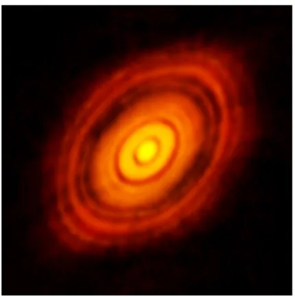
In early 2000’s, Subaru telescope implemented Coronagraphic Imager with Adap- tive Optics (CIAO), which veils the central bright object (i.e., protostar) and can highlight the structure around the protostar (or circumstellar disk). However, since the researchers only observed the scattered light from the surface of the disk, they could not understand the detailed the properties of circumstellar disks. This is because the protoplanetary disk has a large optical depth in the near-infrared wavelength (Subaru Telescope). Figure 1.1 shows the observation of the circumstellar structure around AB Aur (Fukagawa et al., 2004). Similar observations were done in some other protostars and the researchers directly confirmed the disk-like structure. Therefore, from these observations, we can confidently say that the protostars really possess the protoplanetary disk.

The ALMA telescope is completed at 2012. Then, recent ALMA observations have showed surprising images of protoplanetary disks. The most striking observation is the existence of several rings in the protoplanetary disk around HL Tau (Figure 1.2).

(9)

Figure 1.1. Subaru Observation of the circumplanetary disk around AB Aur (Fuka- gawa et al. 2004. Credit: ALMA ESO/NAOJ/NRAO). Central black circle is CHAO which masks the bright central star. Orange region corresponds to the protoplanetary disk.

Although there are many explanation and scenario of the origin of the gaps and the rings seen in Figure 1.2, the most plausible explanation is the existence of (proto or forming) planets. When a protoplanet exists in a protoplanetary disk, the planet can scatter gas particles around the protoplanetary orbit (although part of the gas is absorbed by the protoplanet). Thus, it is considered that the ring naturally appears in the circumstellar disk when the protoplanet exists. Therefore, the several rings may be a proof of the existence of the several protoplanets. In summary, now, we may just observe the stage of planet formation.

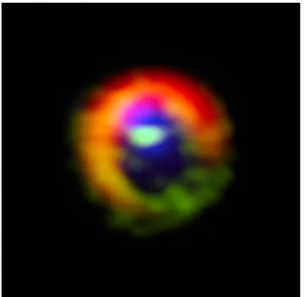
Also, a gap and a stream were observed in the protoplanetary disk around HD142527 using ALMA telescope (Fig. 1.3, Casassus et al. 2015). We can see a clear gap around

(10)

Figure 1.2. Circumstellar disk around protostar HLTau. Several gaps and rings are clearly seen. (Credit: ALMA ESO/NAOJ/NRAO)

the central bright object and the bridge between the central object and the outer disk-like structure. Although the origin of the gap and the stream have not been identified by the observation, some studies predicted that the protoplanet can create the gap or hole around the central protostar. In addition, the outer disk continues to supply the gas to the protoplanet through the stream seen in the gap.

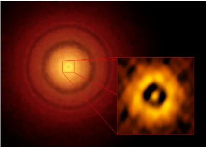
More recently, several rings and two streams were observed using ALMA telescope (TW Hydrae; Figure 1.4). In Figure 1.4, we can see several rings in a large scale, while the gap and stream can be seen in a small scale (the inset of Fig. 1.4). Thus, TW Hydrae also may show the planet formation stage.

Some protoplanetary disks show the gap and spiral structure (SEEDS project).

These disks were called the transitional disk just after its discovery, because it is considered that they are the disks during the gas depletion phase. However, recent

(11)

Figure 1.3. The distribution of gas and dust around protostar HD142527. Two disks are clearly seen the outer and inner disks. The gas streams also can be seen between the outer and the inner disks. The gap (the region between the inner and outer disks) may be formed by the protoplanet. The protoplanet is expected to be located in the gas stream. Credit: ALMA (ESO/NAOJ/NRAO), S. Casassus et al.

observations and theoretical studies imply that the protoplanet can produce the gap and spiral structure during its formation stage.

An exo-planet was found with the radial velocity method at 1995 for the first time as mentioned above. Then, three exoplanets were directly observed at 2008. Figure 1.5 shows an example of the direct observation of exo-planet. In the figure, the exo-planet is oriented toward the north west side.

So far, some exo-planets were confirmed by direct imaging observations (http://exoplanet.eu/). However, we have not observed the forming planets yet. To establish the planet formation scenario or planet formation process, we

(12)

Figure 1.4. The protoplanetary disk around TW Hydrae. Zoomed image are inset. In a large scale, several rings exist. In a very small scale, the gap and gas flow (streams) are confirmed, and they are considered to be formed by the gas-giant planets. (ALMA / ESO / NAOJ / NRAO)

Figure 1.5. Direct observation of Planet orbiting GJ504 (Crejit:NAOJ)

(13)

inevitably need to confirm forming planets or circumplanetary disks. Sallum et al.

(2015) found that Hα emission in a protoplanetary disk (LKCa 15). Without considering the protoplanet and circumplanetary disk, it is diﬃcult to emit such a line in the protoplanetary disk. Thus, it is interpreted as a proof of the accretion luminosity onto the protoplanet or circumplanetary disk.

Thus, although there are some indirect proofs of the forming planet in the circumstellar disk, we have no observation of direct proof on it. As described above, the protoplanet is too small to be directly observed even in near future observations. In- stead, we may able to observe the circumplanetary disks formed around protoplanet by current telescopes. However, we do not know the properties of the circumplanetary disk. Thus, we need to predict it in theoretical or numerical studies.

1.2 Theoretical works

There exist some star forming regions near the sun. Several hundreds of stars are born in each star forming region and the star forming condition have been clearly observed by radio telescopes. Observations indicate that stars form in the molecular cloud core which typically has a size of ∼ 10⁴AU and ∼ 1M_⊙. In molecular cloud cores, since the gravitational energy dominates the thermal, rotational and magnetic energies, the gravitational collapse occurs to form a protostar. After the cloud collapse begins, the cloud isothermally contracts. Then, the dust thermal emission becomes optically thick and the collapsing gas behaves adiabatically and the first adiabatic core forms. Since the first core slowly contracts and the collapsing timescale becomes shorter than the rotation timescale, the magnetic field lines are strongly twisted and the outflow appears from the first core. In addition, the magnetic braking eﬀectively transfers the angular momentum outward. On the other hand, the magnetic field dis- sipates inside the first core, because the ionization degree becomes extremely low and Ohmic dissipation becomes eﬀective in a dense gas region. Therefore, both Lorentz and centrifugal forces weaken and further contraction is promoted.

When the number density of the collapsing cloud (or the contracting first core) ex- ceedsn >10¹⁵cm⁻³, the molecular hydrogens are dissociated and the second collapse occurs. After the dissociation of molecular hydrogen is completed, the gas behaves adiabatically again. Then, the gas contraction stops and the protostar appears (Lar-

(14)

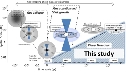
Figure 1.6. Schematic view of star formation in collapsing cloud. The gas accretion and circumstellar disk formation stage are also presented.

son 1969, Masunaga & Inutsuka 2000). The remnant of the first core remains even after protostar formation, and it evolves into the circumstellar disk (Bate, 1998). Af- ter protostar formation (gas collapsing phase), the lump of gas firstly accretes onto the circumstellar disk. Then, although a part of the gas is ejected by the protostellar outflows and jets, the remainder gradually moves toward the central protostar in the circumstellar disk. The star formation scenario expected by recent theoretical studies is summarized in Figure 1.6.

As seen in Figure 1.6, the circumstellar (or protoplanetary) disk is gravitationally unstable in the early phase of the star formation. However, as the protostellar mass increases, the disk becomes stable against the gravitational instability (Toomre, 1964).

The planet formation is expected to occur in such a stable disk.

The standard scenario of planet formation is schematically presented in Figure 1.6.

As seen in the figure, the protoplanetary disk is composed of gas and solid components (dusts). The dusts settle into the equatorial plane and planetesimals form. The planetesimals grow by collision and the earth-like (rocky or icy) protoplanets form. After the mass of protoplanet exceeds about 10 earth mass, the protoplanet cannot main- tain its massive gas envelope due to strong gravity of protoplanet and the runaway

(15)

Protostar Protoplanetary disk(gas＋dust)

Dust layer

Planetesimal

Rocky Planet Planetesimal

Gas Planet and Circumplanetary disk

Figure 1.7. Schematic view of planet formation.

gas collapse begins (Mizuno et al. 1978, Mizuno 1980, Ikoma et al. 2000). In the runaway gas collapsing phase, the circumplanetary disk is expected to be formed because the accreting gas has an angular momentum. Thus, multi-dimensional simulations are necessary to investigate the gas-giant planet formation. Using multi-dimensional simulations, the gas-planet formation was studied (Miyoshi et al. 1999, Lubow et al.

1999, Kley et al. 2001, D’Angelo et al. 2003, Tanigawa & Watanabe 2002). As described above, we need to understand the properties of circumplanetary disk in order to identify the forming planet (or protoplanet) in observations. However, the circumplanetary disk was not fully resolved in two (Tanigawa & Watanabe, 2002) and three (D’Angelo et al., 2003) dimensional simulations due to limitation of the CPU perfor- mance at those days. Using three-dimensional simulations, Machida (2009), Machida et al. (2008, 2010), Ayliﬀe & Bate (2009) managed to resolve the circumplanetary disk.

(16)

However, since their studies focused on the Jovian or Saturn orbit in our solar system, it is diﬃcult to apply their results to other planetary systems. Recently, Gressel et al. (2013) studied the gas-giant planet formation with the state-of-art simulations, in which the magnetic field and its dissipation process were considered. However, they also assumed the Jovian orbit to apply the gas opacity and magnetic resistivity of the protoplanetary disk. Thus, their results are not applicable to other orbits or other planetary systems.

1.3 Aim of this study

Recent observations imply the planet formation in the protoplanetary disk, while yet we have no smoking gun of the planet formation or forming planet even in protoplanetary disks observed by the newest telescopes. The protoplanet cannot be spatially resolved by current and future telescopes, while the circumstellar disks are able to resolve in near future (or current) observations. Thus, we need to theoretically understand the properties of the circumstellar disks in various planetary systems before the observations. However, so far, only a few studies focused on the formation and evolution of the circumplanetary disk. In addition, these studies limited the giant planet formation to Jovian or Saturn orbit in our solar system. Thus, when the general properties of circumplanetary disks are identified from a theoretical study, we can compare them taken from the theoretical study with observations. Therefore, I would unveil the planet formation in various planetary systems.

(17)

Chapter 2

Model for Numerical Simulation

In this chapter, after describing the basic equations used in simulations, I transform it into the non-dimensional form. We cannot calculate the entire protoplanetary disk and time evolution of the protoplanet because we need to spatially resolve the protoplanetary disk, circumstellar disk, and protoplanet. The spatial scale of the protoplanetary disk, circumstellar disk and protoplanet is ∼ 100AU, ∼ 0.1AU and

∼10⁻⁴AU, respectively. Thus, diﬀerence in spatial scale between protoplanetary disk and protoplanet is about 10⁷. In addition, the timescale among them is considerably diﬀerent. Thus, I use the local Hill coordinate, in which only a local region around the protoplanet is calculated using the Hill approximation as mentioned below, and a quasi-steady solution is calculated. I assume a standard model of the protoplanetary disk and the Keplerian motion of the protoplanet. In the Hill approximation, the Hill radius controls the mass and orbit of the protoplanet.

2.1 Fluid motion around a planet embedded in a protoplanetary disk

Let us consider a inviscid isothermal fluid around a protoplanet embedded in a protoplanetary disk. I define a local Cartesian coordinate with the origin at the planet, which rotates in circular orbit around a central protostar with the Keplerian velocity on the equatorial plane of the protoplanetary disk. In the coordinate, the x-, y-, and z-axis corresponds to the radial, azimuthal, and vertical direction of the protoplanetary disk, respectively. The basic equations in the coordinate are described

(18)

as ∂v

∂t + (v· ∇)v =−∇P

ρ − ∇φ_eﬀ −2Ω_pe_z×v, (2.1)

∂ρ

∂t +∇ ·(ρv) = 0, (2.2)

where ρ, t, v, p, φeﬀ, and ez are the gas density, gas velocity, gas pressure, eﬀective potential, and the unit vector in the z-axis, respectively. The gas self-gravity is ignored in this study, because the gravity of protostar and protoplanet dominate the gas-selfgravity. The Keplerian angular velocity of the protoplanet Ωp is given by

Ωp=

√ GMc

r_p³ , (2.3)

where G is the gravitational constant, Mc is a stellar mass, and rp is the distance of a protoplanet from the central star. I adopt an isothermal equation of state

P =c²_sρ, (2.4)

where cs is a constant sound speed, and I assume an optically thin disk.

The eﬀective potential φ_eﬀ is given by

φ_eﬀ =φ_c+φ_rot+φ_p, (2.5)

where φc, φrot, and φp are the gravitational potential of the central star, the orbital centrifugal potential, and the gravitational potential of protoplanet respectively.

These potentials are defined by,

φc = −Ω²_pr³_p

√(rp+x)²+z², (2.6)

φ_rot =−Ω²_p (x²

2 +r_px )

, (2.7)

φ_p = −GM_p

√x²+y²+z², (2.8)

in which the curvature of the protoplanetary disk is neglected. I expand φc around the origin and ignore the third and the higher-order terms. Addingφ_rot to φ_c, I can obtain

φ_c+φ_rot =−Ω²_p (

r²_p+ 3x² 2 − z²

2 )

. (2.9)

(19)

The first term of the right-hand side can be neglected because it is constant. Note that I set the origin as the position of the protoplanet (i.e., r_p = 0). Substituting equation (2.9) into equation (2.5), I can obtain an approximate expression of the eﬀective potential φeﬀ as

φ_eﬀ =−Ω²_p

2 (3x²−z²) +φ_p. (2.10)

2.2 Unperturbed state of the protoplanetary disk

As an unperturbed disk state, I assume a disk without protoplanet. The disk rotates with the Keplerian motion and is in a hydrostatic equilibrium in the vertical direction. I use this unperturbed disk model as the initial condition. In the local Cartesian coordinate, the fluid velocity of the unperturbed disk can be described as

v0 = (

0,−3

2Ωpx,0 )

, (2.11)

in which the y-direction of the velocity originates from the Keplerian rotation of the protoplanetary disk. The equation of motion in thez-direction can be written as

c²_s ρ0

∂ρ₀

∂z =−GMcz[

(rp+x)²+z²]₋3/2

, (2.12)

where ρ0 is the gas density of the protoplanetary disk. Integrating this equation, I have the density distribution in the vertical direction

ρ₀ = Σ0

√2πHexp (

− z² 2H²

)

, (2.13)

where Σ₀ is the surface density of the protoplanetary disk and defined by Σ0 ≡

∫ _∞

−∞

ρ0 dz, (2.14)

and H is the scale height of the protoplanetary disk ^*1 , and defined as H = cs

Ω_p. (2.15)

*1This definition of the scale height is√

2times smaller than the standard value, but this form is often used in non-dimensionalization for convenience.

(20)

The sound speed of gas is given by c_s =

√ k_BT µmH

, (2.16)

where kB, T, µ, and mH are Boltzmann constant, the temperature, the mean molecular weight, and the mass of a hydrogen atom, respectively. Assuming the thermal equilibrium between the disk gas and the dust, I have

T = 280 ( L

L_⊙

)1/4( rp

1 [AU]

)₋1/2

[K], (2.17)

where L and L_⊙ are the protostellar and solar luminosities.

2.3 Non-dimensionalization

In order to transform the equations described in section 2.1 into a dimensionless form, we scale the length by H, the time by Ω⁻¹_p , and the density by Σ₀/r_H, where r_H is the Hill radius given by

rH =rp

( Mp

3M_c )1/3

. (2.18)

Thus, the basic equations of (2.1), (2.2), (2.4), (2.8), and (2.10) are rewritten as

∂ˆv

∂tˆ+ (ˆv·∇ˆ)ˆv = −1 ˆ ρ

∇ˆPˆ−∇ˆφˆ_eﬀ −2ˆz×v,ˆ (2.19)

∂ρˆ

∂ˆt + ˆ∇ ·( ˆρv) = 0,ˆ (2.20)

Pˆ = ˆρ (2.21)

ˆ

φ_p = −3ˆr³_H

√xˆ²+ ˆy²+ ˆz², (2.22)

ˆ

φeﬀ = −1

2 (3ˆx² −zˆ²) + ˆφp, (2.23) where the circumflex denotes nondimensional variables. The relations between Hill radius and the planetary mass are shown in figure 2.1. The gravity of the planet dominates that of the protostar inside the radius rH. The unperturbed nondimensional

(21)

velocity and density are described as vˆ0 =

( 0,−3

2x,ˆ 0 )

, (2.24)

and

ˆ

ρ0 = 1

√2π exp (

−zˆ² 2

)

. (2.25)

As a result, three parameters Mp, Mc, and rp can be removed from the original equations, and I can characterize the models using only one parameter rˆH. Note that a dimensional sound speed is required to convert a non-dimensional length into dimensional one. In addition, dimensional surface density has to be defined as a model of protoplanetary disk when we discuss about a value related to the dimensional density.

(22)

20 40 60 80 100 120 140 160 180 200 Orbital Radius [AU]

5 10 15 20 25 30

Hill Radius [AU]

Dimentional Hill Radius in Constant Planet Masses

0.01 M_Jup 0.1 M_Jup 1 M_Jup 10 M_Jup

10^-1 10⁰ 10¹ 10²

Orbital Radius [AU]

1 2 3 4 5 6 7 8

Hill Radius [Non Dim.]

Non-dimentional Hill Radius in Constant Orbital Radii

Figure 2.1. Relations between Hill radius and the planetary mass. Dimensional and non-dimensional values are plotted in the top and bottom panel. When the planet mass is fixed, the non-dimensional Hill radius increases as the orbital radius increases.

(23)

Chapter 3

Numerical Method

A circumplanetary disk is expected to be significantly smaller than the Hill radius of its own host planet. Thus, we need a very huge telescope to observe the protoplanet or length scale comparable to the planetary radius. On the other hand, in simulations, we need to resolve a few period of the spiral density waves in the circumplanetary disk, which is induced by the interaction between the protoplanetary disk and the protoplanet. Then, we also need a high spatial resolution even in numerical simulations. To realize the high spatial resolution around the protoplanet, I use the nested grid method (e.g. Machida et al. 2008, Matsumoto & Hanawa 2003).

3.1 Initial condition

The initial density profile is adopted as ˆ

ρ(ˆz) = ˆρ_init(ˆz) = max( ˆρ_sky,ρˆ₀(ˆz)), (3.1) whereρˆ_sky is a cutoﬀ density and is set asρˆ_sky= 1.5×10⁻⁶ which corresponds to the value of ρ0 at zˆ= 5. The limitation is required to avoid an unusual low density in a high altitude. Note that the disk density exponentially decreases as the distance from the equatorial plane increases (eq. 2.25). The limitation is a bit artificial. However, this limitation is realistic because the protoplanetary disk is enclosed by the infalling envelope which has a relatively high density.

For the initial velocity profile, I adopt the unperturbed disk velocity (v_x, v_y, v_z) = (0,−3x/2,0). As described below, the initial velocity is described by the non-

(24)

dimensional form.

3.2 Boundary conditions

Considering the symmetry of the equations (2.19), (2.20), (2.21), and (2.23) in the x- and y-axis, I adopt the rotational symmetry in the density and velocities as

ˆ

ρ(ˆx,y,ˆ z) = ˆˆ ρ(−x,ˆ −y,ˆ z),ˆ ˆ

v_x(ˆx,y,ˆ z) =ˆ −vˆ_x(−x,ˆ −y,ˆ z),ˆ ˆ

v_y(ˆx,y,ˆ z) =ˆ −vˆ_y(−x,ˆ −y,ˆ z),ˆ ˆ

v_z(ˆx,y,ˆ z) = ˆˆ v_z(−x,ˆ −y,ˆ zˆ),

(3.2)

and the mirror symmetry at the velocity in the z direction as ˆ

v_z(ˆx,y,ˆ z) =ˆ −vˆ_z(ˆx,y,ˆ −zˆ), (3.3) wherevˆ_x,vˆ_y, andˆv_z arex-,ˆ y-, andˆ z-component of gas velocity. With these boundaryˆ conditions, my computations are executed only in the region of

0≤xˆ≤Lˆx, (3.4)

−Lˆ_y/2≤yˆ≤Lˆ_y/2, (3.5)

0≤zˆ≤Lˆz, (3.6)

where the Lˆx, Lˆy, and Lˆz are the length of the computational domain in x-,ˆ y-,ˆ and z-axis, respectively. I impose the computational boundary atˆ xˆ = 0 and zˆ = 0 considering the symmetry described above.

The boundary conditions of the density and velocity are ρˆ= ˆρinit and vˆ = ˆv0 at x = L_x and z = L_z. The periodic boundary condition is imposed in the y direction as ρ(ˆˆ x,Lˆy/2,z) = ˆˆ ρ(ˆx,−Lˆy/2,z)ˆ and v(ˆˆ x,Lˆy/2,z) = ˆˆ v(ˆx,−Lˆy/2,z).ˆ

3.3 Simulation code

In order to obtain the required spatial resolution near the protoplanet, I use the nested grid method. This method can yield a high spatial resolution, locally gen- erating multiple nested grids. Except for the innermost grid, each grid contains a high-resolution grid, in which the spatial resolution is doubled with the increment of the grid level. In the original nested grid code, each grid has the same number

(25)

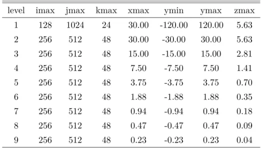
Table 3.1. Number of cells in each axis and the boundary positions of the nested regions

level imax jmax kmax xmax ymin ymax zmax

1 128 1024 24 30.00 -120.00 120.00 5.63

2 256 512 48 30.00 -30.00 30.00 5.63

3 256 512 48 15.00 -15.00 15.00 2.81

4 256 512 48 7.50 -7.50 7.50 1.41

5 256 512 48 3.75 -3.75 3.75 0.70

6 256 512 48 1.88 -1.88 1.88 0.35

7 256 512 48 0.94 -0.94 0.94 0.18

8 256 512 48 0.47 -0.47 0.47 0.09

9 256 512 48 0.23 -0.23 0.23 0.04

of computational cells and the same rectangular shape. To optimize this study, I improved the code, in which a diﬀerent aspect ratio of each cell and each grid is al- lowed. The first grid level (i.e. root grid, l = 1) has the cells of (128×1024×24) in the x-, y-, and z-directions, respectively. On the other hand, the second and higher level of grids (l ≥ 2) have cells of (256×512×48). The grid level, the number of cells and non-dimensional length scales in each direction used in the simulations are summarized in Table 3.1.

The Roe numerical solver (Roe, 1981) is used for the time integration of equations of hydrodynamics and an adaptive time step method is used. In this method, a time step is individually determined in each grid level. Hence, the finer grid requires a large number of integrations because of the Courant-Friedrichs-Lewy (CFL) condition.

3.4 Model parameters

Model parameters are summarized in table 3.2 which lists the model name, non- dimensional Hill radius, maximum grid level, planet mass at 5.2 AU, non-dimensional and dimensional minimum spatial resolutions and elapsed time until the end of the calculation. The model name is composed of two parts: the Hill radius and maximum

(26)

grid level. Among the models, the models containing T are the standard model that have a maximum grid levell_max = 6−9. On the other hand, models H064R7 (l_max = 7) and H064R9 (l_max = 9) are made by checking the results with diﬀerent resolutions.

The dimensional planet masses shown in the table are derived from equations (2.15), (2.16), (2.17), and (??), assuming M_c =M_⊙, L=L_⊙, and µ= 2.34.

Table 3.2. Model Parameters

Model name rˆ_H l_max M_p/M_Jup(5.2AU) ∆ˆx(l_max) ∆x/r_Jup Time [Ω⁻¹]

H135T6 1.35 6 1.00 7.3×10⁻³ 4.1 163.47

H115T7 1.15 7 0.62 3.7×10⁻³ 2.1 40.29

H100T7 1.00 7 0.41 3.7×10⁻³ 2.1 43.01

H087T7 0.87 7 0.27 3.7×10⁻³ 2.1 87.69

H077T8 0.77 8 0.19 1.8×10⁻³ 1.0 31.68

H070T8 0.70 8 0.14 1.8×10⁻³ 1.0 26.99

H064T8 0.64 8 0.11 1.8×10⁻³ 1.0 45.09

H054T8 0.54 8 0.06 1.8×10⁻³ 1.0 35.94

H036T9 0.36 9 0.02 9.2×10⁻⁴ 0.5 24.56

H064R7 0.64 7 0.11 3.7×10⁻³ 2.1 21.64

H064R9 0.64 9 0.11 9.2×10⁻⁴ 0.5 24.09

3.5 Sink cell method

In simulations, since the protoplanet is located at the origin, the gravity of cells around the origin is extremely strong. Thus, the calculation is often broken or the long-term time integration does not work well. To avoid such situations, in various studies, a softening parameter ε, which ‘softens’ the gravity in the vicinity of the protoplanet, is adopted to the gravitational potential as

φ^′_p = −GMp

√x²+y²+z²+ε². (3.7)

However, this technique is not suﬃciently justified and causes unrealistic results near the protoplanet. Thus, the more plausible way to avoid the singularity is required to

(27)

precisely calculate the circumplanetary disk.

The most straightforward way is to resolve the surface of a protoplanet with a suﬃciently high spatial resolution and remove the gas accreted on the surface every time step. However, this treatment is wasteful for my purpose. Machida et al. (2008, 2010) already mentioned this problem, and they determined the sink radius, in which the gas inside the sink radius is removed from the computational domain. This is an appropriate way for my purpose. However, since they did not discuss the amount of mass to be removed, we cannot evaluate the validity of their method. The amount of removing mass would significantly influence the structure of circumplanetary disk because the balance among the accretion flow and the outflow determines the structure in the vicinity of the protoplanet. Therefore, the correct estimation of the amount of the removed mass is crucially important.

In the simulation with the sink method, the removed gas should be determined by the pressure gradient force because I do not change the gravity of the protoplanet with a softening parameter. Thus, I need to appropriately treat the gas pressure (or pressure gradient force) when the sink method is implemented. In addition, I also need to pay attention to the gas flow in the vicinity of the protoplanet or around the sink. Obviously, the gas density and pressure are the highest at the origin (i.e., at the position of the protoplanet). Thus, the region around protoplanet (or around the origin) would have a positive pressure gradient force in the radial direction. However, from the simulation, I cannot confidently determine the gas density (and the gas pressure) at the origin because the spatial resolution is not suﬃcient to resolve the protoplanet. Thus, instead of adopting the density derived from the simulations, I extrapolate the density (or the pressure) at the origin using the density in the vicinity of the cell as

ˆ

ρs:i,j = [6 ˆρi+1,j −4 ˆρi+2,j + ˆρi+3,j

+ 6 ˆρ_i,j+1−4 ˆρ_i+1,j+1+ ˆρ_i+2,j+1

−4 ˆρ_i,j+2+ ˆρ_i+1,j+2 + ˆρ_i,j+3]/4,

(3.8)

where i and j are the identified numbers of the sink cells located at (ˆx,y,ˆ zˆ) = (∆x/2,∆y/2,∆z/2). In this interpolation, density distribution in the vertical (or z) direction is neglected, because I confirmed the steeper gradient of dρ/dˆˆ z in the vertical direction than that in the x and y direction on the equatorial plane.

(28)

There is an another sink cell at(ˆx,y,ˆ z) = (∆x/2,ˆ −∆y/2,∆z/2), and the treatment is the same but the position rotates 90 degree with respect to the origin. At every time step of the simulations, I replace the density derived from the simulation into that is extrapolated by the cells around the protoplanet as

ˆ

ρ^′ = min ( ˆρ,( ˆρs+ ˆρ)/2). (3.9) If a steady state exists, the density of sink cell would converge to a constant value with time. Note that without the averaging of right hand side of equation (3.9), I confirmed that the computation has crushed.

(29)

Chapter 4

Convergence Analysis of the Simulations

The simulation or the time-integration can continue until the simulation has crashed. Thus, I need to determine the epoch at which the simulation stops. The criterion of stopping the simulation diﬀers from one study to another. For example, Tanigawa et al. (2012) stopped their computation when the accretion flow onto the circumplanetary disk comes to a nearly steady state. On the other hand, Szulágyi (2017) continued to run the computations until the planetary gap profile comes to a steady state. To evaluate the structure of the circumplanetary disk, I need to execute the computation until the disk becomes a steady state. However, previous studies could not show a steady state of the circumplanetary disk. This is because in such studies the simulations were performed with a softening parameter ε or smoothing length, as mentioned above.

The softening or smoothing length enables to avoid singularity of the planet s gravitational potential at the origin and can yield realistic flow in a large scale formed by gravitational interaction, but accumulates a mass infinitely around the planet.

Consequently simulations cannot be reached steady state and we would extremely overestimate the accreted mass and the size of circumplanetary disk

In this thesis, I developed a new sink method and confirmed a steady state of circumplanetary disk and convergence of physical quantities. I remove the mass of the cells every time steps in the finest grid, in which an amount of the removed gas is dynamically determined in the simulation. When the circumplanetary disk achieves

(30)

a steady state, the removed mass is equal to the mass captured by the protoplanet in the protoplanetary disk. Then, the physical quantities of the circumplanetary disk are converged. In this chapter, I show the results of the convergence test and discuss the validity of the steady state derived from my sink method.

4.1 Overview of mass distributions on the equatorial plane

Figure 4.1 shows the density distribution at the end of the simulation (the epoch is listed in Table 3.2) on the mid-plane for each model which has a diﬀerent parameter of the Hill radius. As the Hill radius decreases, the radius of dense gas region, which corresponds to a circumplanetary disk, rapidly decreases. This figure also shows two pairs of spiral arms which can be observed for models with the Hill radius larger than ˆ

r_H≥0.77 (Figs. 4.1[a]–[e]). The density of the spiral arms is higher than that of the other regions. However, for models with smaller Hill radii (ˆrH<0.77), the spiral arms are not clear compared with models with larger rˆH. In addition, the root of arms are away from the origin or apart from each other.

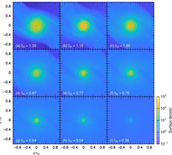
Figure 4.2 shows the surface density distributions for each model, which is calculated as

Σ(x, y) =

∫ H

−H

ρ(x, y, z)dz. (4.1)

The area of dense region (the region with yellow color in Fig. 4.1) decreases as the Hill radius decreases. Although this tendency is similar to the density distribution on the equatorial plane, the dense spiral arms seen in the density distribution in models with rˆ_H = 0.87 and 0.77 (Fig. 4.1[d] and [e]) do not appear in Figure 4.2(d) and (e).

Thus, the dense arms are considered to be induced only near the mid-plane, while weak spiral arms are expected to appear in the region above the mid-plane. Note that although the Hill radius for models in Figure 4.2(a) is larger than that for model with Figure 4.2(b), the maximum density in the larger Hill radius model is lower than that in the higher Hill radius model. This implies that the spatial resolution aﬀects the density distribution. This kind of the resolution dependency was reported in some previous studies (e.g. Morbidelli et al. 2014).

(31)

–0.8 –0.4 0 0.4 0.8

–0.8 –0.4 0 0.4 0.8 –0.8 –0.4 0 0.4 0.8 –0.8 –0.4 0 0.4 0.8 –0.8

–0.4 0 0.4 0.8

(a)ˆr_H= 1.35 (b)ˆr_H= 1.15 (c)rˆ_H= 1.00

–0.8 –0.4 0 0.4 0.8

(d)ˆr_H= 0.87 (e)ˆr_H= 0.77 (f)ˆr_H= 0.70

y/rH

x/r_H –0.8

–0.4 0 0.4 0.8

–0.8 –0.4 0 0.4 0.8 (g)ˆr_H= 0.64

–0.8 –0.4 0 0.4 0.8 (h)ˆr_H= 0.54

–0.8 –0.4 0 0.4 0.8

10^–1 10⁰ 10¹ 10² 10³ 10⁴

Gasdensity

(i)ˆr_H= 0.36

Figure 4.1. Gas density (color) on the equatorial plane around the protoplanet at the end of the simulations. Parameter rˆH diﬀers in each panel.

4.2 Convergence of cumulative mass

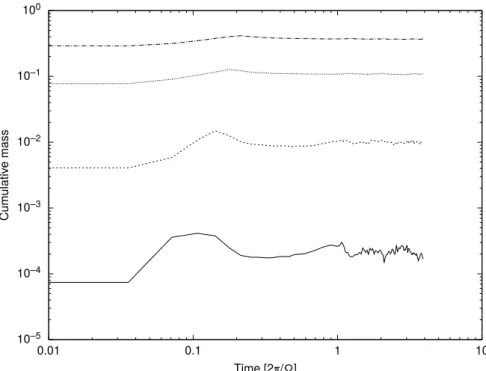
In order to evaluate convergence of the calculations, the time sequence of the mass distribution is examined. Figure 4.3 shows time evolution of the cumulative mass within a radius Rand scale height H for model withrˆ_H = 0.64. The cumulative mass is calculated as

M_cd(R) =

∫ R 0

∫ 2π 0

∫ H

−H

ρ(x, y, z)dzdθdr, (4.2)

where r is defined as r = √

x²+y², and θ is the azimuthal angle measured from the x-axis. In this figure, the cumulative masses at four diﬀerent radii R = rH/100,

(32)

–0.8 –0.4 0 0.4 0.8

–0.8 –0.4 0 0.4 0.8 –0.8 –0.4 0 0.4 0.8 –0.8 –0.4 0 0.4 0.8 –0.8

–0.4 0 0.4 0.8

(a)ˆr_H= 1.35 (b)ˆr_H= 1.15 (c)rˆ_H= 1.00

–0.8 –0.4 0 0.4 0.8

(d)ˆr_H= 0.87 (e)ˆr_H= 0.77 (f)ˆr_H= 0.70

y/rH

x/r_H –0.8

–0.4 0 0.4 0.8

–0.8 –0.4 0 0.4 0.8 (g)ˆr_H= 0.64

–0.8 –0.4 0 0.4 0.8 (h)ˆr_H= 0.54

–0.8 –0.4 0 0.4 0.8

10^–1 10⁰ 10¹ 10² 10³

Surfacedensity

(i)ˆr_H= 0.36

Figure 4.2. Surface density Σˆ distribution near the protoplanet at the end of the calculation for each model.

r_H/10, r_H/2 and r_H are plotted by the solid, dashed, dotted, and dash-dotted line, respectively.

After the calculation starts, the cumulative masses steeply increase and show a weak peak. Then, they converge to a constant value within an orbital period (<2πΩ⁻¹).

The time to converge the cumulative mass is suﬃciently shorter than the growth timescale of the planet. This indicates that the density enhancement due to the growth of the protoplanet greatly aﬀects the structure of the circumplanetary disk. In addition, the density distribution of the circumplanetary disk changes in a short time compared with the Keplerian timescale. Since the growth timescale of the protoplanet is much longer than the Keplerian timescale, this simulation can be regarded as a snapshot of the accreting circumplanetary disks.

(33)

Cumulativemass

Time [2π/Ω]

10^–4 10^–3 10^–2 10^–1 10⁰ 10¹

0.01 0.1 1 10

Figure 4.3. Time evolution of the accreted mass within a radiusRˆ and scale height H for model withrˆ_H= 0.64. The solid, dashed, dotted, and dash-dotted line represents the non-dimensional mass withinRˆ = ˆrH/100,rˆH/10,rˆH/2, andrˆH, respectively. The elapsed time is normalized by the orbital period.

Figure 4.4 is the same plot as in Figure 4.3 but for model with rˆH= 0.36which has the smallest Hill radius in this study. The figure shows that cumulative masses have weak (overshooting) peaks before they converge to a constant value. The time scale for the convergence in this model is shorter than that for model withrH = 0.64. This implies that a smaller protoplanet quickly changes its surrounding structure. Thus, even for the models with a smaller Hill radius, I can regard it as a snapshot around a growing planet. However, for model with rˆ_H = 1.35 (Fig. 4.5) which has the largest Hill radius among the models, I cannot confirm a clear convergence of the cumulative masses within the computation time. In Figure 4.5, although top three lines, which corresponds to R ≥ r_H/10, show a peak, they continue to decrease. On the other hand, the cumulative mass forR=rH/100 (the bottom line) also show a peak, while it keeps an almost constant value. This indicate that the radiusR=rH/100is located within the inner edge of circumplanetary disk. Although the cumulative masses seen

(34)

Cumulativemass

Time [2π/Ω]

10^–5 10^–4 10^–3 10^–2 10^–1 10⁰

0.01 0.1 1 10

Figure 4.4. Time evolution of the accreted mass within a radiusRand scale height H for model withrˆ_H= 0.36. The solid, dashed, dotted, and dash-dotted line represents the non-dimensional mass withinRˆ = ˆrH/100,rˆH/10,rˆH/2, andrˆH, respectively. The elapsed time is normalized by the orbital period.

in Figure 4.6 also have not been completely converged, the mass within R < rH/100 keeps a constant value for ˆt ≳ 0.2. Thus, a steady state is expected to be achieved around the protoplanet (or inside the circumplanetary disk).

4.3 Overview of azimuthal velocity distribution on the equatorial plane

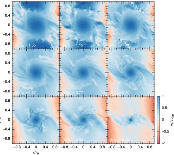
Figure 4.7 shows the azimuthal velocity distribution on the equatorial plane normalized by the local Keplerian angular velocity of the protoplanet, which is given by

ˆ vKep =

√

3ˆr³_Hr,ˆ (4.3)

for each model at the end of the calculation. The figure shows that the normalized azimuthal velocities are constant near the protoplanet, which indicates that the gas

(35)

Cumulativemass

Time [2π/Ω]

10^–3 10^–2 10^–1 10⁰ 10¹ 10²

0.01 0.1 1 10 100

fluid around the protoplanet moves according to the Keplerian motion. Outside a critical radius, which is defined as the boundary between the circumplanetary disk and the protoplanetary disk, the normalized velocities are still positive, while fluid shows a turbulent motion. This feature indicates that the angular momentum transfer occurs around the critical radius. Also, the critical radii normalized by the Hill radius increase as the Hill radii increase for models.

The azimuthally averaged azimuthal velocity is calculated by

¯ vθ(ˆr) =

∫r+∆ˆˆ r ˆ r−∆ˆr

∫2π

0 Lˆzdθdˆr

∫ˆr+∆ˆr r−∆ˆˆ r

∫2π

0 rˆρ dθdˆˆ r

, (4.4)

and is shown in Figure 4.8 for models with rˆH= 0.36, 0.64, 1.00, and 1.35, in which the velocity is normalized by the Keplerian angular velocity. For each model, the region near the protoplanet has almost the Keplerian velocity, while the normalized velocity steeply decreases in the region far from the protoplanet. Gressel et al. (2013)

(36)

Cumulativemass

Time [2π/Ω]

10^–3 10^–2 10^–1 10⁰ 10¹ 10²

0.01 0.1 1 10

defined the inflection point of the radial profile using the time averaged specific angular momentum and reported that the circumplanetary disk has a radius of 0.5ˆrH. Although the tendency seen in Figure 4.7 is similar to their result, the decreasing point of the normalized velocity (or the size of the circumplanetary disk) clearly de- pends on the Hill radius (or the normalized Hill parameter). Therefore, my results implies that the outer edge of circumplanetary disk has a similar dynamical structure for models with diﬀerent Hill radii.

4.4 Convergence of azimuthal velocity

Convergence of the azimuthal velocity is also investigated. Figures 4.9 and 4.10 shows the time sequences of the normalized azimuthal velocity at four diﬀerent radii for models with rˆH = 0.36, and 1.35. The azimuthal velocity converges near the

(37)

–0.8 –0.4 0 0.4 0.8

–0.8 –0.4 0 0.4 0.8 –0.8 –0.4 0 0.4 0.8 –0.8 –0.4 0 0.4 0.8 –0.8

–0.4 0 0.4 0.8

(a)ˆr_H= 1.35 (b)ˆr_H= 1.15 (c)rˆ_H= 1.00

–0.8 –0.4 0 0.4 0.8

(d)ˆr_H= 0.87 (e)ˆr_H= 0.77 (f)ˆr_H= 0.70

y/rH

x/r_H –0.8

–0.4 0 0.4 0.8

–0.8 –0.4 0 0.4 0.8 (g)ˆr_H= 0.64

–0.8 –0.4 0 0.4 0.8 (h)ˆr_H= 0.54

–0.8 –0.4 0 0.4 0.8 –1 –0.5 0 0.5 1

vθ/vKep

(i)ˆr_H= 0.36

Figure 4.7. Normalized azimuthal velocity distribution for each model at the end of the calculation. The coordinate is scaled by rˆH.

protoplanet, while it oscillates the region far from the protoplanet. Nevertheless, the amplitudes in the oscillation are not very large, which implies that the azimuthal velocity roughly converges in all the radii. The region showing almost constant azimuthal velocity in Figure 4.9 is located inside the critical radius, as seen in Figure 4.7(i).

4.5 Summary

In this chapter, I showed the convergence of cumulative mass and azimuthal velocity, i.e. specific angular momentum. Cumulative masses show convergence except for model with rˆH = 1.35. In addition, all the azimuthal velocities profiles are con-

(38)

Averagedazimuthalvelocity

ˆ r/ˆr_H ˆ

r_H= 0.36 ˆ r_H= 0.64 ˆ r_H= 1.00 ˆ r_H= 1.35 0

0.2 0.4 0.6 0.8 1

0.001 0.01 0.1 1

Figure 4.8. Radial profiles of the averaged azimuthal velocity on the equatorial plane.

The velocity is normalized by the Keplerian velocity. Radial distances are also normalized by the Hill radius.

verged. Thus, I can check the validity of the simulation and confidently analysis the circumplanetary disk in the subsequent chapters.

(39)

Azimuthalvelocity

Time [2π/Ω]

r/r_H= 0.01 r/r_H= 0.10 r/r_H= 0.50 r/r_H= 1.00

–0.4 –0.2 0 0.2 0.4 0.6 0.8 1

0.01 0.1 1 10

Figure 4.9. Time sequences of the azimuthal velocity on the mid-plane for model with ˆ

rH = 0.36 at diﬀerent radii. The velocities and radial distances are normalized by each Keplerian velocity and the Hill radius, respectively.

(40)

Azimuthalvelocity

Time [2π/Ω]

r/r_H= 0.01 r/r_H= 0.10 r/r_H= 0.50 r/r_H= 1.00 –0.4

–0.2 0 0.2 0.4 0.6 0.8 1

0.01 0.1 1 10

Figure 4.10. Time sequences of the azimuthal velocity on mid-plane for model with ˆ

rH = 1.35 at diﬀerent radii. The velocities and radial distances are normalized by each Keplerian velocity and the Hill radius, respectively.

周惑星円盤の典型的半径と惑星質量に対する依存性