17
Revisiting Income Elasticities
in Food Demand from
an Age Perspective
Hiroshi Mori, Kimiko Ishibashi
and Dennis Clason
Part I. Cross-Sectional Approach:
Since 1970, the Japanese government has spent roughly US $ 60
1
billion on rice acreage conversion/curtailment programs, $ 2.0± billion
each year, in vain (MAFF, various issues). Ill retrospect, per Capita
rice consumption peaked in 1965 and has been consistently declining. Policy makers backed by the farm interests have never been certain if this declining tendency would continue as the economy keeps growlng.
They on many occasions hoped that per capita consumption had hit the
bottom line.18
Table 1. Estimates of elasticity of expenditure on selected food groups with respect to living expenditure (≒income) , 2000 and 2003,
as reported by FZES 2000 2 ElasticityT-Value 之ニ7F宥稗ユfヌVR Allfood 緜33紊B0.6630ー47 Rice ゅ3B0.214.89 Bread 緜s纉"0.6712.46 Noodles 紊R繝r0.488.93 Freshfishandshellfish 經C經"0.519.53 Freshmeat 縱C偵20.7519.47 Fluidmilk 經C"縱R0.5715.48 Eggs 經縱"0.5211.16 FreshVegetables 經R0.4612.32 Fresh fruit 紊B緜0.314.44 Eating-out B經"1.3116.64
AlcoholicbeVerage 3b紊0.568.30
Sources: Bureau of Statistics, Family Income and Expendituyle Surue_V, 2000 and
2003, Appendix Table 4.
What is the problem here? In more concrete terms, what has
caused the apparent discrepancies between time-series and
cross-sec-tional observations? Let us dig into the problem, using a simple hypo-thetical case of commodity x, in place of rice.
Small children aged under 5 generally eat much less food, say
70% less on average than teenagers who may eat as much as the
ordinary adults. If so, some sorts of age modification, by such as "adult
equivalence scales" as a common practice, should be undertaken to determine the realistic estimates of income elasticity of demand for
impera-Revisiting income Elasticities iII Food Demalld from an Age Perspective 19
Table 2. Hypothetical cases of commodity x consumption by 2 groups
of 4 person households headed by young and middle-aged adults: BasicData 陪6VニD67VラヤW6VニHuFR tionofCommodityX (kg/year)(1000yen/year) HouseholdA: HHaged30andspouse 2childrenageunder5
Totalhousehold HouseholdB: HHaged45andspouse c#S
2×10 2teenagers
Totalhousehold 鼎C
AVerageilーCOmeelasticity: Noagemodification 茶Cモ#b梯イウ#bイSモ#S梯イSウ#S瀞ウ縱B
AVerageillCOmeelasticity: Age1110dificationby "aduttequiValellCeSCales" 茶CモC梯イウCイSモ#S梯イSウ#S噸
Notes: Age modifications with an assumption of adult equivalence scales for a child ullder 5 and teenager-0.3 and 1.0, respectively, resulting in modified
household consulllption: 20+6/0.3-40 for hotlSellOld A and 20+20/1.0-40 for
household B.
tive especially il一 the country like Japan where the seniority-based
wages prevail in the labor market. A simple illustration is presented in
Table 2 above.
In an actual setting, further caution should be recognized, i. C., if average consumption within the adult population varies significantly by age and cohort, either generational or geographical, then what proce-dures should or could be taken?
In cross-sectional analyses, uslng micro-data, Various
20
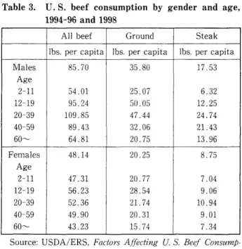
Table 3.日.S. beef consumption by gender and age,
1994-96 and 1998 Allbeef 背&襭Steak lbs.percapita 免'2W&6友lbs.percapita
Males Age 2-ll 塔R縱35.80 r經2
54,01 Rr6.32 12-19 涛RB50.05 %R 20-39 偵コ47.44 B縱B 40-59 塔偵C232.06 紊2 60- 田B繝20.75 2纉b Females Age 2-ll 鼎ゅB20.25 唐縱R 47.31 r7.04 12-19 鉄b228.54 湯b 20-39 鉄"b21.74 ウ釘 40-59 鼎偵2().31 湯 60- 鼎2215.74 途BSource: USDA/ERS, Factors Ajfecting U. S. Beef Consump-tion, October 2005, p. 19.
race are incorporated (Cox and Wohlgenant, 1986; Blaylock and Smalレ
wood, 1986; Blundel, Pashardes, and Weber, 1993; Perali and Chavas,
2000; Blisard, Variyam, and Cromartie, 2003).
Here is a very recent survey data showing per capita beef
consumption by gender and age in the United States (Table 3).
Consumption in the form of ground beef is the highest in the age group, 12-19, in both males and females and steak consumption is the highest
in the age group, 20-39, and it declines toward the higher age groups.
Will ground beef consumption tend to decline and steak
consump-tion increase as the total U. S. populaconsump-tion ages in the next decades?
In most USDA projections since 1980S (Blaylock and Smallwood,
Revisiting Income Elasticities il一 Food Demand from an Age Perspective 21
that if a person moves from one demographic group to another, she/he
will immediately take on the characteristics prevalent in the new group.
In other words, cohort effects are ignored in most of these studies. If a man ages from his young-adulthood of 20-39 to the middle age of 40 -59, his consumption of ground beef, for example, is supposed to decline from 47.4 1bs. to 32.1 1bs. in the above case of beef consumption in the
United States.
In any cross-sectional analysュs Which covers a short span of time, it is almost impossible to detect cohort effects in one's consumption
behavior. To our knowledge, economists at the USDA have never
officially attempted to compare consumption by age across different
time-periods, say the late 1990S, the late 1980S, and the 1970S, maybe
because the available data are not complete in consistency and classifi-cations.
In a developed economy or a long stagnated society like pre-war
Japan, human food consumption may change only gradually in
accord-ance with caloric need and the ability to digest, as one ages from
childhood to adulthood and elderliness. In developing economies,
however, today's young are not the same as their counterpart of yesterday and won't be the same as today's elderly when they grow old
within the next few decades. The food consumption habits formed
when people come of age will be retained to some extent or another
throughout their lives. Cohort effects may be negligible with some food
products and in some societies, but it has been found that they play significant roles in determining one's consumption of such staple foods
as rice and fish in Japan (Isibashi, 2004; Mori and Clason, 2004; Mori et
22
Cohort effects will be discussed in the latter half of this paper.
We would like to come back to the first topic, i. e" howto deal withthe
demographic factors in cross-sectional analysts, uSlng panel data. Inlarge cross-sectional analysis, it is customary to app一y demographic
dummy variables, such as household head is black; household owns the
house; number of persons, 13 to 18 years of age, etc. (Cox and
Wohle-genant, 1986; Dong et a1.,1998; Browning and Chiappori, 1998; Dong et
a1., 2004). In determining the relationship of income and individual food demand, One of the crucial questions is how to take scale economies
into consideration, i.e., is a 5 person- household 20 % worse off than a
4 person-household with the same household income? ; more specifi-cally, "what expenditure level would make a family with three chi一dren
as well off as it would be with two children and $ 12,000?"(Pollack and
Wales, 1981, p. 1533) In view of the fact that food is entirely "private
good", scale economies could be ignored from the analysis of individualproducts (Deaton and Paxson, 1998, p. 899). In determining the effects
of household income onindividt.1al food consumption, however,
econ-omies of scale should come explicitly into the picture.
Instead of introducing a number of demographic dummy vari-ables, we first classify households by the type of households such as a married household in which househo一d head (HH) is in the 30s with 2
children aged under 10; a married household in which HH is in the 60s
with no dependent and the like. In doing so, we can circumvent the
problems of "equivalence scales" in individual food consumption as well
as scale economies in household incomes. We then regress household
consumption of individual food products, rice, fresh pork, fresh beef,Revisiti11g lncollle Elasticities il一 Food Demalld from an Age Perspective 23
data into per capita basis here, because we are dealing with the same categories of household).
We have conducted these investigations for selected years from
the mid 1980s to 2001, using approximately 96,000 monthly panel data (8,000 × 12) each year. We have come across numerous problems, which
include zero purchases and "outliers"inobservations. Many econo・
mists emphasize the importance of appropriate treatment of non-con-suming households based on their belief that the household deliberately chooses not to consume particular goods given its current budget and
the prices it faces (Dong et aL1998, p. 472; Perali and Chavas, 2000, p.
1022). In the case of rice in Japan, however, the vast majority of
households consume rice almost every day. Zero purchases by as many
as 45 % of the survey households in particular months may simply mean
that they have stocks from purchases done in the previous months.
Therefore, we do not so far see the need for"Amemiya-Tobin
approach" for the censored demand systems, for example (Dong et a1.,
2004; Yen et a1., 2003).
Outliers are most problematic in the case of rice and fresh fruit. In some subset of data which averages 15kg of rice per household per
mollth, a purchase of 360 kg is reported. Intuitively this may represent
"outlier" which should be deleted from the analysis to avoid possible
biases. Then how about 40 or 50kgP Most analysts knowledgeable of
Japanese food consulTlption may agree that 90kg should represent otltliers, though. 0111y tentatively, we have excluded the data which
exceed 3 times of mean values* of all the observations in the each subset classified by the household type (* excluding zero purchases in
24
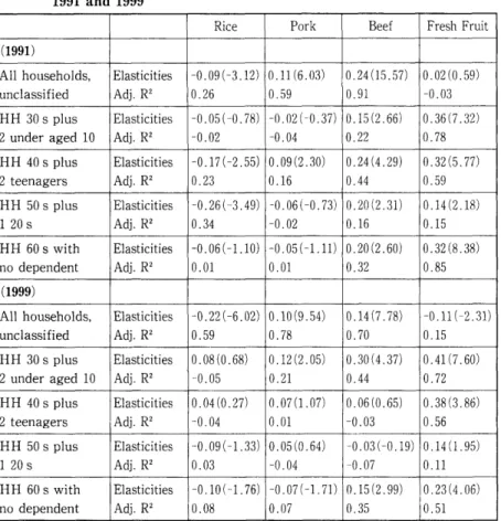
Table 4. Cross-sectional regression estimates of income elasticities of aト home consumption of rice, fresh pork, fresh beef, and fresh fruit, 1991 and 1999
Rice イBeef 波&W6'V唯
(1991) Allhouseholds, 之ニ7F友妨2-0.09仁3.12) 貳ツッ20.24(15.57) "經鋳 unclassified F「"0.26 經0.91 蔦2 HH30splus 之ニ7F友妨2-0.05仁0.78) 坪モr0.15(2.66) bビ" 2underaged10 F「"-0.02 蔦B0.22 縱 HH40splus 之ニ7F友妨2-0.17(-2.55) 茶"0.24(4.29) "コ縱r 2teenagers F「"0.23 b0.44 經 HH50splus 之ニ7F友妨2-0.26仁3.49) 啌モiモ縱20.20(2.31) Br 120S F「"0,34 蔦"0.16 R HH60swith 之ニ7F友妨2-0.06(-1.10) 蔦Rふ貳ツ0.20(2.60) "モr nodependent F「"0.01 0.32 繝R (1999) Allhouseholds, 之ニ7F友妨2-0.22(-6.02) ヲ經B0.14(7.78) 蔦モ" unclassified F「"0.59 縱0.70 R HH30splus 之ニ7F友妨20.08(0.68) "R0.30(4.37) 紊ビ緜 2underaged10 F「"-0.05 0.44 縱" HH40splus 之ニ7F友妨20.04(0.27) rr0.06(0.65) 握3ッ 2teenagers F「"-0.04 -0.03 經b HH50splus 之ニ7F友妨2-0.09(-1.33) Xャ3cB-0.03仁0.19) B纉R 120S F「"0.03 蔦B-0.07 貳ツ HH60swith 之ニ7F友妨2-0.10仁1.76) 蔦yfモ縱0.15(2.99) 2ィb nodepeltdent F「"0.08 r0.35 經
Note: Figures in parentheses denote卜values.
Sources: Computations by Ishibashi, National Agricultural Research Center, Tsu-kuba, Japan.
Following the traditional lead of Prais and Houthakker (1971),
we use the group average figures classified by anntlal household
Revisiting Income Elasticities in F。od Demand from an Age Perspective 25
i.e., by every half million yen (US $ 4,500) or one million yen, or every
1,000 households from the lowest to the highest income groups, for
example. In doing so, both top and bottom 5 % households in annual
income are excluded.The results for 199l and 1999 are shown in Table 4. When all the
households of approximately 96,000 each year are analyzed on a simple per capita basis without considerations to demographic factors such as
family size and household composition, rice is found to be
income-negative, pork and beef income-positive, and fresh fruit income-negative
or irresponsive. When the households are classified by household type,
rice is generally found income-negative, and beef income-positive, the
same as in the non-classified approaches. Pork, however, is found income-neutral and most strikingly, fresh fruit definitely
income-posi-tive. These findings from the classified approaches better conform to
our intuition nourished from the daily observations.
Part II. Time-Series Approach:
In 1979, the Bureau of Statistics started to publish age-related
consumption data in its annual reports of Family Income and
Expendi-ture Survey. In the past two decades or so, per capita household consumption of rice has beell consistently declining from 45 to 30kg,
that of fresh pork, excluding processed llleat, has only slightly declilled
from 5.4 to 5.0kg, that of fresh beef on the constant rise ulltil 1996 from
2.4 to 3.6kg, when the e-coli 0-157 was detected in fresh beef on the
market, and that of fresh fruit declining as fast as the case of rice from
45 to 31kg, as shown in Table 5.
Revisltmg Income Elasticities in Food Demand from al一 Age Perspective 27
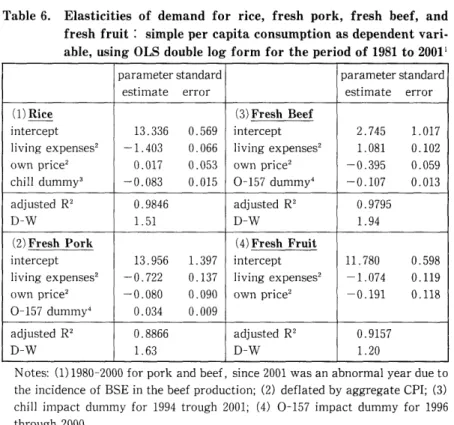
Table 6. Elasticities of demand forrice, fresh pork, fresh beef, and
fresh fruit : Simple per capita consumption as dependent vari-able, using OLS double log form for the period of 1981 to 20011
parameterstandard estimateerror parameterstandard estimateerror
津 illterCept 23c經c(3)里王旦吐旦堅至 intercept 縱CSr liVmgeXpenSeS2 蔦紊3cbliVlngeXpenSeS2 " ownprlCe2 sS2ownprlCe2 蔦鉄S
chilldummy3 蔦R0157dummy4 蔦s2
adjustedRZ 纉イbadjustedR2 纉s迭D-W 經D-W 纉B
(2)FreshPork illterCept 2纉Sc途(4)FreshFruit intercept 免ツ縱經唐
livlngeXpenSeS2 蔦縱##3rHVlllgeXpe11SeS2 蔦sC
ownprlCe2 0-157dummy4 蔦3CownprlCe2 蔦
adjustedR2 繝ツbadjustedR2 纉Sr
D-W 緜2D-W
Notes: (1)1980-2000 for pork and beef, since 2001 was an abnormal year due to the illCidence of BSE in the beef production; (2) deflated by aggregate CPI; (3)
chill impact dummy for 1994 trough 2001; (4) 0-157 impact dummy for 1996
through 2000.
steadily during the 1980s until the "bubble" burst in 1991 from 0.96 to 1.
16million in 2000 constant yel一 Which has been followed by the decade
long recession. Real price of rice was stable for a decade and half until
1994 when the domestic rice production was hit by the devastatingly
chilly summer, and its price has been falling steadily since then. Real
prlCe Of pork kept falling during the 1980s from 197 to 135 yen per 0.1
kg and has been leveled off in the 1990S. That of beef has been on the
28
moderately with a slight (10 %) increasing trend, as is shown in
Table5.
When all these economic factors taken into consideration in the
traditional approach of time-series regression analysis, the estimates of income and prlCe elasticities of demand for these four products are
determined as shown in Table 6.
Elasticities of demand with respect to living expenditure (as
proxy for income) for rice are estimated aレl.4, that for pork, beef and fresh fruit, respectively at -0.7, 1.1 and -1.1,with significantトvalues for all products. Setting aside the absolute magnitude of elasticities, the estimates for rice, negative, and that for beef, positive, may be
acceptable, when compared to the results of cross-sectional analysis in
the previous section (Table 4, in particular). The negative estimate for
pork, as highas -0.7 is questionable, and what's more, a negative 1.i
elasticity for fresh fruit is highly questionable, however. Intuitively, the
premise that a 10 % increase in income will lead to a ll % decrease in
fruit consumption, ceteris paribus, can not be accepted. Across the
countries, fresh fruit is generally deemed to be "normal good" (Seal et
a1., 2003).
In what follows, We will examine the changes in fresh fruit consumption in Japan from the demographic perspectives.
Table 7 shows changes in household consumption of fresh fruit
by the age groups of household head (HH) for the past 20 years since
1980. The average household consumption gradually declined from
159.Okg in 1980 to 120.5kg in 1990 and thento 102.7kgin 2000. Twenty
years ago, households headed by those in the 20s and the early 30s
Revisitlng Income Elasticities in Food Demand from an Age Perspective 29
Table 7. Household consumption of fresh fruit by age groups of household
head (HH), 1980, 1985, 1990, 1995, and 2000
(kg/year) HHage 塔1985 涛1995AVerage S偵135.1 #絣108.4 "縒
~24 都"51.8 "紕54.1 b縒 25-29 "縒74.6 鼎b39.1 "綯 30-34 3R綯99.4 都纈52.7 鼎"繧 35-39 cB綯127.5 涛ゅ71.3 田 40-44 s142.6 偵93.2 都偵 45-49 s"繧152.7 3R112.0 涛" 50-54 sB綯145.8 #偵121.9 繧 55-59 cゅb148.7 3偵2128.1 #縒 60-.64 cR繧149.5 C133.5 3綯 65- c140.5 C137.6 3ゅSources: Family Income and Ehenditure Survey, various issues.
by those in the 50s and 60S. In 2000, the young households of HH 20s
alld the early 30s consumed as much as 70 % less fresh fruit than the
older households. The households of HH 20s and 30s have decreased
fresh fruit consumption much faster than the older households headed
by the 50s and 60S. This is what the Japanese government's 1994 White
Paper on Agriculture described as "wakamono no kudamono-banara"
(leaving off fresh fruit by the young).
Clearly, the pattern of consumption by age, "age-consumption
profile" is not fixed over time. One thing should be kept in mind in
comprehending this table. Those in their late 20s in 1980 have aged to
their late 30s in 1990 alld their late 40s in 2000, for example. Reading
Table 7 diagonally, Japanese consumers of fresh fruit seem to carry the
eating habits formed during their youth into their lives in later years.
This is called "cohort effects" in human behavior. The question to be
30
The household heads in their early 30s in 1980 have aged to their
late 40s in 1995. They were born il一 the late 1940s and may have shared the similar experience as they came of age, and thus they belong to thesame generational cohort. If the household survey does not trace the
same subjects over time, those household heads in the age group, 25-29 in 1980, those in 35-39 in 1990 and those il一 45-49 in 2000, respectively,
for example, can be regarded as the same (generational) cohort. But their household consumption does not represent their
con-sulllptlOn alone, containing the consumption by their dependents who
live with them. Typically, there were two infants in 1980, two
teen-agers in 1990 and one or two young adults in 2000, if they still lived with
parents. Individual consumption by these dependents should have changed substantially, quite likely much more so than their parents
over time as they grew up. Therefore, the simple per capita figures
derived from dividing household consumption by the number of persons in the respective households do not represent the individual consump-tion by age for these cohorts.
Mori and lnaba (1997) designed a unique method of deriving per
capita consumption by individual household members from household
data classified by HH age groups, which is not explained in full in this
paper (refer to the Master thesis by M. Lewis, 1997 0r paper by M. Lewis,
H. Mori, and Wm. D. Gorman, 1997). Very simply, it is a mechanical
process shown below:
Suppose we have 2 Observations, 025 and Q50, compiled from a
sufficient number of panel data, relatillg tO household consumption by
age of household head (HH), 25 and 50 years of age, respectively.
問 。 〈 在 片 山 口 何 回 口
n o
ヨ
ω
巴
g
z
巳 己g
z
p
u
o
己 ロ
m H U m ロ 門 二 吋 Oヨ
ω
ロ〉m m
印 刷 】m
w
司印H u m w
n
片 山 〈 。Family c
o
m
p
o
s
i
t
i
o
n
by age groups o
f
h
o
u
s
e
h
o
l
d
head
,
1
9
9
1
3
2
where
X
id
e
n
o
t
e
s
a
v
e
r
a
g
e
i
n
d
i
v
i
d
u
a
l
consumption by p
e
r
s
o
n
,
i
y
e
a
r
s
o
f
a
g
e
.
I
f
we c
a
n
assume t
h
a
t
i
n
f
a
n
t
s
,
a
g
e
z
e
r
o
,
do n
o
t
consume t
h
i
s
p
r
o
d
u
c
t
,
t
h
e
n
,
X
2Si
s
a
u
t
o
m
a
t
i
c
a
l
l
y
d
e
t
e
r
m
i
n
e
d
a
t
.
1
0
,
and
X
osa
t
3
.
5
(
(
8
-1
)
/
2
)
.
I
n
t
h
e
r
e
a
l
i
t
y
,
t
h
e
c
a
l
c
u
l
a
t
i
o
n
i
s
n
o
t
t
h
i
s
s
i
m
p
l
e
,
b
e
c
a
u
s
e
t
h
e
f
a
m
i
l
y
c
o
m
p
o
s
i
t
i
o
n
m
a
t
r
i
c
e
s
by HH
a
g
e
g
r
o
u
p
s
a
r
e
v
e
r
y
complex a
s
i
s
shown i
n
Table 8
.
Those who a
r
e
i
n
t
e
r
e
s
t
e
d
i
n
t
h
e
p
r
o
c
e
d
u
r
e
s
a
r
e
a
d
v
i
s
e
d
t
o
r
e
f
e
r
t
o
Lewis e
t
a
.
l
'
s
p
a
p
e
r
above mentioned a
s
a
b
e
g
i
n
n
e
r
'
s
g
u
i
d
e
and Tanaka e
t
a
.
l
(
2
0
0
4
)
f
o
r
t
h
e
l
e
s
s
b
i
a
s
e
d
and t
h
e
more s
o
p
h
i
s
t
i
開c
a
t
e
d
e
s
t
i
m
a
t
o
r
s
.
When t
h
e
t
a
b
l
e
c
o
n
t
a
i
n
i
n
g
p
e
r
c
a
p
i
t
a
i
n
d
i
v
i
d
u
a
l
c
o
n
s
u
m
p
t
i
o
n
by
a
g
e
g
r
o
u
p
s
f
o
r
r
e
s
p
e
c
t
i
v
e
y
e
a
r
s
o
v
e
r
a
c
e
r
t
a
i
n
p
e
r
i
o
d
o
f
t
i
m
e
,
c
o
h
o
r
t
t
a
b
l
e
(
T
a
b
l
e
9
)
i
s
a
v
a
i
l
a
b
l
e,
we can decompose c
h
a
n
g
e
s
i
n
consumption
by a
g
e
i
n
t
o
t
h
e
e
f
f
e
c
t
s
o
f
a
g
e
(
i
n
a
narrow s
e
n
s
e
)
,
g
e
n
e
r
a
t
i
o
n
a
l
c
o
h
o
r
t
,
and “
p
u
r
e
"
t
i
m
e
,
by means o
f
c
o
h
o
r
t
a
n
a
l
y
s
i
s
.
I
n
t
h
i
s
s
t
u
d
y
,
we u
s
e
N
akamura's B
a
y
e
s
i
a
n
c
o
h
o
r
t
model (N akamura,
1
9
8
6
)
b
a
s
e
d
on i
n
t
u
i
-t
i
v
e
l
y
r
e
a
s
o
n
a
b
l
e
a
s
s
u
m
p
t
i
o
n
o
f
“
z
e
n
s
h
i
n
t
e
k
i
henka" (
g
r
a
d
u
a
l
c
h
a
n
g
e
s
between s
u
c
c
e
s
s
i
v
e
p
a
r
a
m
e
t
e
r
s,
.
i
e
.,
a
g
e
g
r
o
u
p
s
4
0
-
4
4
and 4
5
-
4
9
may
n
o
t
a
b
r
u
p
t
l
y
d
i
f
f
e
r
i
n
b
e
h
a
v
i
o
r
;
t
h
o
s
e
born i
n
t
h
e
l
a
t
e
1
9
6
0
s
s
h
o
u
l
d
n
o
t
be d
r
a
s
t
i
c
a
l
l
y
d
i
f
f
e
r
e
n
t
from t
h
o
s
e
born i
n
t
h
e
e
a
r
l
y
1
9
7
0
s,
f
o
r
exam-p
l
e
)
.
担 当 日 印
E
H
M
m
z
n
0
5
0
E
S
己 巳 片 山m
w
凹 吉 司0 0
己 口 。 ョ ωロ 己 守 o ヨ 間 口 〉m m
叩 苛 巾 百 円 U O の 片 山 〈 。E
s
t
i
m
a
t
e
s
o
f
i
n
d
i
v
i
d
u
a
l
at-home consmnption o
f
f
r
e
s
h
f
r
u
i
t
by age
,
1979-2001
,
kg/year
3
4
-R
e
v
i
s
i
t
i
n
g
I
n
c
o
m
e
l
E
a
s
t
i
c
i
t
i
e
s
i
n
F
o
o
d
Demand f
r
o
m
a
n
Age P
e
r
s
p
e
c
t
i
v
e
3
5
Table 1
1
.
E
l
a
s
t
i
c
i
t
i
e
s
o
f
demand f
o
r
r
i
c
e
,
f
r
e
s
h
pork
,
f
r
e
s
h
beef
,
and f
r
e
s
h
f
r
u
i
t
:
(
A
)
s
i
m
p
l
e
p
e
r
c
a
p
i
t
a
consumption a
s
dependent v
a
r
i
a
b
l
e
(
r
e
p
l
i
c
a
o
f
Table 6
)
and
(
B
)
p
e
r
i
o
d
e
f
f
e
c
t
s
p
l
u
s
grand mean d
e
r
i
v
e
d
from cohort
analy~s
i
s
a
s
dependent v
a
r
i
a
b
l
e
,
estimated using OLS double log
form f
o
r
the p
e
r
i
o
d
o
f
1
9
8
1
t
o
2
0
0
1
1(A)
d
e
p
e
n
d
e
n
t
v
a
r
i
a
b
l
e
ニ)
B
(
d
e
p
e
n
d
e
n
t
v
a
r
i
a
b
l
e
=
s
i
m
p
l
e
p
e
r
c
a
p
i
t
a
c
o
n
s
u
m
p
t
i
o
n
p
e
r
i
o
d
e
f
f
e
c
t
s
+
g
r
a
n
d
mean
(
1
)
R
i
c
e
p
a
r
a
m
e
t
e
r
s
t
a
n
d
a
r
d
e
r
r
o
r
p
a
r
a
m
e
t
e
r
s
t
a
n
d
a
r
d
e
r
r
o
r
e
s
t
i
m
a
t
e
e
s
t
i
m
a
t
e
i
n
t
e
r
c
e
p
t
1
3
.
3
3
6
0
.
5
6
9
1
1
.
8
4
3
0
.
5
9
5
l
i
v
i
n
g
e
x
p
e
n
s
e
s
2
-1.
4
0
3
0
.
0
6
6
-1.
1
3
4
0
.
0
7
3
own p
r
i
c
e2
0
.
0
1
7
0
.
0
5
3
-
0
.
0
2
5
0
.
0
4
9
c
h
i
l
l
d
ummy
3-
0
.
0
8
3
0
.
0
1
3
-
0
.
0
6
9
0
.
0
1
3
a
d
j
u
s
t
e
d
R
2
0
.
9
8
4
6
0
.
9
7
2
6
D-W
.
1
5
1
.
1
6
1
(
2
)
F
r
e
s
h
p
o
r
k
i
n
t
e
r
c
e
p
t
1
3
.
9
5
6
1
.
3
9
7
1
1
.
4
1
9
2
.
1
5
6
l
i
v
i
n
g
e
x
p
e
n
s
e
s2
-
0
.
7
2
2
0
.
1
3
7
-
0
.
9
8
1
0
.
2
1
2
own p
r
i
c
e2
-
0
.
0
8
0
0
.
0
9
0
-
0
.
1
3
9
0
.
1
3
9
0
-
1
5
7
dummy4
0
.
0
3
4
0
.
0
0
9
0
.
0
5
0
0
.
0
1
4
a
d
j
u
s
t
e
d
R
2
0
.
8
8
6
6
0
.
8
4
1
6
D-W
.
1
6
3
0
.
9
6
(
3
)
F
r
e
s
h
b
e
e
f
i
n
t
e
r
c
e
p
t
2
.
7
4
5
.
1
0
1
7
-1.
1
3
2
0
.
9
2
0
l
i
v
i
n
g
e
x
p
e
n
s
e
s
2
.
1
0
8
1
0
.
1
0
2
0
.
9
9
3
0
.
0
9
2
own p
r
i
c
e2
-
0
.
3
9
5
0
.
0
5
9
-0
4
.
0
8
0
.
0
5
4
0
-
1
5
7
dummy4
-
0
.
1
0
7
0
.
0
1
3
-
0
.
1
0
2
0
.
0
1
2
a
d
j
u
s
t
e
d
R
2
0
.
9
7
9
5
0
.
9
8
2
0
D-W
.
1
9
4
.
1
4
1
(
4
)
F
r
e
s
h
f
r
u
i
t
i
n
t
e
r
c
e
p
t
1
1
.
7
8
0
0
.
5
9
8
3
.
0
4
6
0
.
5
2
1
l
i
v
i
n
g
e
x
p
e
n
s
e
s
2
-1.
0
7
4
0
.
1
1
9
0
.
2
7
7
0
.
1
0
3
own p
r
i
c
e2
-
0
.
1
9
1
0
.
1
1
8
-
0
.
3
4
9
0
.
1
0
3
a
d
j
u
s
t
e
d
R
2
0
.
9
1
5
7
0
.
3
2
4
5
D-W
.
1
2
0
2
.
0
1
N
o
t
e
s
:
)
1
(
1
9
8
0
-
2
0
0
0
f
o
r
p
o
r
k
a
n
d
b
e
e
f
;
(
2
)
d
e
f
l
a
t
e
d
by a
g
g
r
e
g
a
t
e
C
P
I
;
(
3
)
c
h
i
l
l
i
m
p
a
c
t
dummy f
o
r
1
9
9
4
t
h
r
o
u
g
h
2
0
0
1
;
(
4
)
0
-
1
5
7
impact dummy f
o
r
1
9
9
6
t
h
r
o
u
g
h
36
Conditions, and the special events such as the incidence of e-coli 0-157
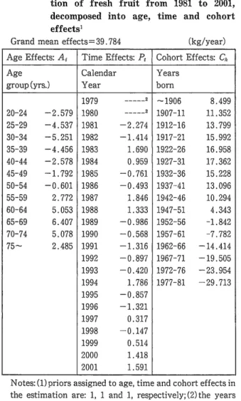
in the case of beef and some vegetables in Japan, for example. In stead of traclng Changes in simple per capita consumption which are confounded with changes due to the demographic factors other than pure economic factors, we will regress "pure" time effects derived from our cohort analysts against changes in income and own
price over the period from 1980 to 2001. Table ll shows our estimates
of "age-free income and price elasticities" of demand for fresh fruit and other products, rice, fresh pork, and fresh beef.
Compared to non-age compensated approach as is shown in
Table 6, We have now obtained positive expenditure (proxy for income)
elasticity of 0.28 for fresh fruit, with卜values close to 3, and own-priceelasticity of -0.35, also with t-value larger than 3.
The drastic decline in per capita consumption of fresh fruit in the
past 2 to 3 decades should have been caused mostly by the demographic factors, i.e., the replacement of fruit eating older cohorts by the newer cohorts who seem to have much less aptitude for fresh fruit, for
unknown reasons. People, including seemingly knowledgeable market and nutrition experts, are quoted to remark, "today's young do not like to soil their hands, peeling skins off," Or they do not know how to use
knife to peel the skin (Asahi, October 23, 2004). They may be totally
mistaken, because mandarin oranges, known as "TV-oranges" (easy to
peel while watchillg TV) has declined the most in consumption and
JapalleSe apples which are generally quite big in size, not good for
eating out of hands without cutting, have kept nearly constant in
consumption, on the colltrary: per Capita consumption of mandarin
38
In this study, We classified household data by household types which involve the age of household head and family size and age
composition, such as a couple plus two teenagers and the like, to
circumvent the problems of age of household members and economies
of scale. We ran the analysis, regressing household consumption of
various food items against household incomes by each household type,
to derive "age and scale economy-free" income elasticities.
We obtained intuitively plausible, positive signs for income
elasticities for fresh fruit. Fresh pork was found income-neutral,instead of definitely positive income elasticites derived from non-age compensated approach.
Theoretically as well as emplrlCally, income elasticities should
vary along the income scales of household, usually taperlng Off toward
the higher end (E. Engel, 1885; Prais and Houthakker, 1971; Saegusa,
1980; Fodder and Trall-Nam, 1994). What we have so far obtained is
plausible slgnS Of elasticities, not their exact magnitude. We have
approximately 96,000 panel data of differing annual household incomes.Consumption data is monthly. Except for bread, fluid milk, and the like
which are commonly purchased on regular basis every week, even those
households which consume in year total much lager quantities of certain products, say rice, or apples than the average, may purchase much smaller amounts, or even zero purchase, in some months.
Depending on how to aggregate individuai household data, We often
obtain the irregular results which can not be supported by the theory.
As already mentioned in the foregoing text, We have to learn the more
practical ways of how to aggregate the data, including the treatment of
zero-PUT-R
e
v
i
s
i
t
i
n
g
I
n
c
o
m
e
E
l
a
s
t
i
c
i
t
i
e
s
i
n
F
o
o
d
D
e
m
a
n
d
f
r
o
m
a
n
A
g
e
P
e
r
s
p
e
c
t
i
v
e
3
9
c
h
a
s
e
s
c
o
u
l
d
d
e
s
e
r
v
e
o
u
r
next c
o
n
s
i
d
e
r
a
t
i
o
n
s
.
I
n
t
h
e
l
a
t
t
e
r
h
a
l
f
o
f
t
h
e
paper
,
we f
i
r
s
t
d
e
r
i
v
e
d
i
n
d
i
v
i
d
u
a
l
p
e
r
c
a
p
i
t
a
consumption o
f
f
r
e
s
h
f
r
u
i
t
by age from t
h
e
h
o
u
s
e
h
o
l
d
d
a
t
a
c
l
a
s
s
i
f
i
e
d
by t
h
e
age groups o
f
h
o
u
s
e
h
o
l
d
head from 1
9
7
9
t
o
2
0
0
.
1
These
d
a
t
a
were t
h
e
n
s
e
p
a
r
a
t
e
d
i
n
t
o
age
,
g
e
n
e
r
a
t
i
o
n
a
l
c
o
h
o
r
t
and time e
f
f
e
c
t
s
,
u
s
i
n
g
N
akamura's Bayesian c
o
h
o
r
t
model
.
The a
g
e
-
f
a
c
t
o
r
compensat-e
d“
p
u
r
e
"
time e
f
f
e
c
t
s
i
n
t
h
e
changes o
f
h
o
u
s
e
h
o
l
d
consumption o
f
f
r
e
s
h
f
r
u
i
t
f
o
r
t
h
e
p
a
s
t
two d
e
c
a
d
e
s
were t
h
e
n
r
e
g
r
e
s
s
e
d
a
g
a
i
n
s
t
income and
p
r
i
c
e
s
o
v
e
r
t
h
e
same p
e
r
i
o
d
.
We o
b
t
a
i
n
e
d
s
t
a
t
i
s
t
i
c
a
l
l
y
s
i
g
n
i
f
i
c
a
n
t
income e
l
a
s
t
i
c
i
t
y
o
f
+
0
.
2
8
,
i
n
s
t
e
a
d
o
f
-1
1
.
o
b
t
a
i
n
e
d
from t
h
e
o
r
d
i
n
a
r
y
,
non-age compensated t
i
m
e
-
s
e
r
i
e
s
a
n
a
l
y
s
i
s
.
This r
e
s
u
t
1
n
o
t
o
n
l
y
b
e
t
t
e
r
a
p
p
e
a
l
s
t
o
o
u
r
i
n
t
u
i
t
i
o
n
b
u
t
a
l
s
o
conforms t
o
t
h
e
e
s
t
i
m
a
t
e
s
from t
h
e
age
f
a
c
t
o
r
-
c
o
n
t
r
o
l
l
e
d
c
r
o
s
s
-
s
e
c
t
i
o
n
a
l
a
n
a
l
y
s
i
s
i
n
t
h
e
f
i
r
s
t
h
a
l
f
o
f
t
h
i
s
p
a
p
e
r
.
End N
o
t
e
s
:
(
1
)
E
x
p
e
n
s
e
s
i
n
J
a
p
a
n
e
s
e
y
e
n
were c
o
n
v
e
r
t
e
d
a
t
t
h
e
e
x
c
h
a
n
g
e
r
a
t
e
o
f
.
1
$
0
=
1
1
0
y
e
n
,
w
h
i
c
h
p
r
e
v
a
i
l
e
d
i
n
t
h
e
l
a
t
t
e
r
h
a
l
f
o
f
1
9
9
0
s
.
The a
c
t
u
a
l
r
i
c
e
paddy
f
i
e
l
d
c
o
n
v
e
r
s
i
o
n
p
r
o
g
r
a
m
s
h
a
v
e
b
e
e
n
s
o
c
o
m
p
l
e
x
t
h
a
t
i
t
may b
e
a
l
m
o
s
t
i
m
p
o
s
s
i
b
l
e
t
o
i
d
e
n
t
i
f
y
a
l
l
t
h
e
e
x
p
e
n
s
e
s
i
n
c
u
r
r
e
d
.
References
A
s
a
h
i
New
ゆ
a
p
e
.'12
0
0
4
.
“
J
a
p
a
n
e
s
e
a
n
d
F
r
叫t
s
,
"
E
v
e
n
i
n
g
E
d
i
t
i
o
n
,
O
c
t
o
b
e
r
2
3
,
p
.
2
.
B
l
a
y
l
o
c
k
,
.
J
,
.
R
a
n
d
D
.
M
.
S
m
a
l
l
w
o
o
d
.
1
9
8
6
.
U
.
S
.
Demand f
o
'1F
o
o
d
:
H
o
u
s
e
h
o
l
d
E
x
t
e
n
d
i
t
u
1
'
e
s
,
D
e
m
o
g
r
a
p
h
i
c
s
,
and P
m
j
e
c
t
i
o
n
s
,
USDA/ERS
,
T
B
-
1
7
1
3
,
F
e
b
r
u
-a
r
y
.
B
l
i
s
a
r
d
,
N
. ,
.
J
N.
V
a
r
i
y
a
m
,
a
n
d
.
J
C
r
o
m
a
r
t
i
e
.
2
0
0
3
.
Food E
>
.
沙問d
i
t
u
1
'
e
s
b
y
U
.
.
s
H
o
u
s
e
h
o
l
d
s
:
L
o
o
k
i
n
g
Ahead
拘2020,
A
g
r
i
c
u
l
t
u
r
a
l
E
c
o
n
o
m
i
c
R
e
p
o
r
t
N
o
.
8
2
1
,
USDAjERS.
40
June, 570-597.
Browning, M. and P. A. Chappori. 1998. "Efficient lntra-Household Allocations: A
General Characterization and Empirical Tests," Econometrica, 66(6),
November, 1241-1278.
Cox, T. L., and M. K. Wohlgenant. 1986. "Price and Quality Effects in
Cross-Sec-tional Demand Analysis," American Journal of Agn-cultural Economics," 68
(3) , August, 908-919.
Davis, C. G. and B-W Lin. 2005. Factws Ajfecting U. S. Beef Consumption, LDP-M
-135-02, USDA/ERS, October.
Deaton, A.and C. Paxson. 1998. "Economies of Scale, tiousehold Size, and the
Demand for Food," Journal of Political Economy, 106(5) , 897-930. Deaton, A. and S. Zaidi. 2002. Guidelines for Constntcting Consumption Agg7,egateS
for Welfare Analysis, Living Standards Measurement Study (LSMS)
Work-ing Paper No. 135, WashWork-ington, D、 C., The World Bank.
Dong, D., ∫. S. Shonkwiler, and 0. Capps, Jr. 1998. "Estimation of Demand Functions Using Cross-Sectional Household Data: The Problem Revisited," AmenAcan Journal of Agn'culturlal Economics, 80 (3) , August , 466-473.
Dong, D., B.W.Could, and H.M.Kaiser. 2004."Food Demand in Mexico: An
Application of the AmemlyaTobin Approach to the Estimation of a
Censored Food System,H Ame77'can Journal of Agn'cultural Economics, 86
(4) , November, 1094-1107.
Engel, Ernest. 1895. "Die Lebenskosten Belgischer Arbeiter-Familien Frtlher und
Jetzt," International Statistics Institute Bulletin, 9, No. 1, 11124.
Ishibashi, Kimiko. 2004. "Changes in Household Rice Consumption by the House-hold Type and Income Level," Journal of Food System Resewch, Vol. ll, 1 -15 (in Japanese).
Japanese Government, Bureau of Statistics, Family Income and Expenditure Stm,ey,
Annual Report, various issues, Tokyo.
Japanese Government, Bureau of Statistics, Famil,v Income and ExPenditu71e Slquey,
Panel Data, various months, Courtesy: Bureau of Statistics through Ministry
of Agriculture, Forestry and Fisheries.
Japanese Government, Ministry of Agriculture, Forestry and Fisheries. 1995. White
Paper on Agn'culture, 1994, Tokyo.
Statistics and Information Department. Statistical Yearbook of Minist7γ Of Agn'culture, Forest7y and FZ'sheries, various issues.
Revisiti11g lncolme Elasticities in Food Demalld from an Age Perspective 41
Mexico State University, Las Cruces, NM, July.
Lewis Hendrickson, M., H. Mori, and Wm. D. Gorman. 2001." Estimating Japanese
At一一holTle Food Consumption by Age Groups while Controlling for lncome
Effects," Cohort Analysis of Japanese F()od Consumption, eds. by H. Mori, 93
-121.
Lin, B-W, J.N.Variyam, J. Allshouse, and J. Cromartie. 2003. Food and Agn'cultu71al
Commodity Consumption in the United States: Looking Ahead to 2020,
Agricultural Economic Report No. 820, USDA/ERS.
Meyerhoefer,C., C, Ranney, and D. Sahn. 2005. "Consistent Estimation of Censored
Demand Systems Using Panel Data," Ame77'can Journal of Agricultural
Economics, 87(3) , August, 6601672.
Mori, Hiroshi (eds.). 2001. Cohort Analysis of Japanese Food Consumption-New
and Old Gene7,ations, Tokyo, Senshu University Press.
Mori, H. and T. Inaba. 1997. "Estimating llldividual Fresh Fruit Consumption by
Age from Household Data, 1979 to 1994," Journal of Rural Economics, Vol. 69(3), 175-85.
Mori, I-L, D. LClason, I.Dyck, and Wm. D. Gorman. 2001."Age in Food Demand
Analysis-A Case Study of Japanese Household Data by Cohort
Approach," Coho71 Analysis of Japanese Food Consumptl'on, eds. by H. Mori,
311-345.
Mori, H., M, Tanaka, and T. Inaba. 2004. "Predicting At-home Consumption of Rice
and Fresh Fish under a Rapidly Aging: A Cohort Approach," The Annual
Bulletin of Socl'al Scz'ence, Vol. 38, Senshu University, 41-62 (in Japanese).
Mori, H.and D.LClason. 2004."Cohort Approach as an Effective MeallS for
Forecasting Consumptiolュin an Aging Society: The Case of Fresh Fruit in
Japan," Senshu Unive?,sity Economic Bulletin, Vol. 38(2), 45-70.
Mori, H. and D. L Clason. 2004. "A CollOrt Approach for Predicting Future Eating
Habits: the Case of At-hollle CoIISLlmption of Fresh Fish alld Meat il一 an Aging Japanese Society," Internatllonal Review of F()Od and Agnlbusiness
Management Rel)lew, Vol. 7(1), 22-41.
Nakamura, Takashi. 1986. "Bayesian Cohort Models for General Cohort Tables,=
Annals of the Insh'tute of Statl'Ldical Mllihematl'cs, Vol. 38, 353-370, Tokyo.
Perali, F. and J-P Chavas. 2000. "Estilllation ()f Censored Demand Equations from Large Cross-Section Data," America Jmmu7l l)I Agriculturtll Economics, 82
(4), November, 1022-1037.
Podder, N. and B. Tram-Nam. 1994. "A New Approach to Estimating Engel
42
262-276.
Pollak, R. A. and T. J. Wales. 1981. "Demographic Variables in Demand Analysis,"
Econometrica, Vol, 49, No. 6 (November) , 1533-1551.
Prais, S. J. and H. S. Houthakker. 1971. The Analysis of Family Budgets, Cambridge at The University Press.
Saegusa, Yoshikiyo. 1986. "Estimating Expenditure Elasticities for Foods from
Concentration Curves," Economy and Economics, No. 58, Tokyo Municipal
University, 1-20.
Tanaka, M., H. Mori and T. Inaba. 2004. "Re-estimating per Capita Individual
Consumption by Age from Household Data," The Japanese Journal of Rwal Economics, Vol. 6, 20130.
Wold, Herman, in Associationwith L Jureen. 1982. Demand Analysis : A Study in
Econometn'cs, reprinted, Westport, Connecticut, Greenwood Press.
Yen, S. T., B-H Lin, and D. M. Smallwood. 2003. "Quasi- and Simulated-Likelihood
Approaches to Censored Demand Systems: Food Consumption by Food Stamp Recipients in the United States," Ame77'can Journal of Agricultural
R
e
v
i
s
i
t
i
n
g
Income E
l
a
s
t
i
c
i
t
i
e
s
i
n
Food Demand from a
n
Age P
e
r
s
p
e
c
t
i
v
e
4
3
APPENDIX
44
いのかもしれない。ただしソフトドリンク消費に関し, Rentz&
「5(りReynolds等(1991)はそうは考えていない。日本の場合は戟後世代でも,
1人当たり肉類消費が3.0kg前後であった1950年代に成人した世代と,
30kgに達した1980年代以降に成人した世代の間には,歴然たる食習慣
の差があってもおかしくない。
同上『経済財政白書』によると, 「コーホート分析とは,年齢階級別の
データが時系列で把握可能な統計を用いて,各データを年齢効果,世代効
莱,時代効果に分ける手法である。ここで(1)年齢効果とは時代や生まれ年
の違いを超えて,年齢階級というライフサイクルに応じた影響を示すもの,
(2)世代効果とは生まれ年の違いによって表れる影響を示すもの, (3)時代効
宋とは,年齢効果や世代効果を超えて景気変動等その時代に各世帯共通に
見られた影響を示すものである」とされる。時代効果にかかわる「登些整
共通に見られた」はなかなか微妙な表現であるが,ここではこの程度の説
明で良しとしよう。
本稿では,内外とも(食料)消費分析に関してはスタートしたばかりの
コウホート分析の動向を歴史的にリヴューし,今後の方向を示唆したい。
(註1) cohortは,三二ホ-トでなく,三ヱホ-トと発音される。従って本稿では,以後コウホ-ト分析と記す。統計数理研究所の関連論文も,コウホ-ト
分析で統一されている.
人口・世帯の年齢構成
Fair andDominguez (1991)は, 「本論文の結果はきわめて剖目すべきである。米国人口の年齢構成変化は消費,住宅投資などに有意な説明力を
持っていることが明らかになった」 「われわれは従って"representative-[1とりagent approachを放棄する」と述べている。 Modiglianiのライフサイク
ル仮説を持ち出すまでも無く,人の(消費)貯蓄行動は成人し,職につき,
「27〕
Revisiting IIIC()me Elasticities in Food Demand from an Age Perspective 45
変化すれば,社会の消費・貯蓄が変化するのは至極当然である。しかしそ
れをモデル化しようとすれば,従来の(代表的)個人の最適化問題から離
れる難しさに直面する。
食料消費に限っても,幼児から思春期を経て成人し,やがて老齢化する
に従い,消費の量と質は顕著に変化する。ベイビーブームで若年層が膨ら
む時代と,やがて人口の高齢化が進む時代では,社会の食料消費が質・量
ともに変化するのは説明を要しない。食料消費を,家計調査等のミクロデ
ータを使ってクロスセクション的に分析する場合も,マクロデータを使っ
て時系列的に分析する場合にも,人口構成が激変している経済では,単に
名目人数で割ったpercapitaデータは, Woldが言うようにバイアスを生
「62〕みやすい。変化が一方向で,定常的であればトレンド項の導入で凌ぐこと
も可能であろう(註2)。しかし現実はそう単純ではないことが多い。
それに対処する正当な方法は,現実の適用例はわが国ではほとんど皆無
〔23〕に近いが, "adult equivalence scales"であった(Lewbel, 1985)。同上 Woldは早くも1953年に, Cap. 14-5のHthe age scale of consumption" のなかで,たとえば男子の0-3, 416, ・・・, 17-18歳の"consumer units" は, 19歳以上を1.0とすると,それぞれ0.1, 0.2, -・, 0.9であるとし
て,家族月数を"consumer units"に換算して各品目の所得弾力性を計測
〔62〕 〔49〕
している。この考えはその後Prais& Houthakkerに引き継がれ(註3),
理論的にも計測面でも, "unit consumer scale", "(adult) equivalence
scales"を巡る出発点となった。
"equivalence scale"には,世帯所得のデフレーターとしての用途と,
食料や燃料など個々の世帯消費を成人1人当たりに換算するための尺度と
しての側面がある。たとえば所得弾力性を計測する場合,前者は分母に,
後者は分子にそれぞれ関わることになる。前者はきわめて具体的には,
Pollack and Wales (1981)の言葉を借りると, 「子供が3人の家族を子46
〔47〕 〔40〕
出が必要か」,より直裁には, Muelbauerのいう"the cost of children"
の問題で,一般化は極めて難しく,理論化の対象になり難い。後者は,住
居費や燃料等の場合はどれだけ「規模の経済が働くか」の問題であるが,
〔12,14」
多くの食料品は, Deaton他によると"entirely private goods"とみなさ
れるから,規模の経済が働く余地は少なく,主として子供たちの生理的要
求と噂好にかかわるものだから,客観的な決定は可能であろう。
決定の仕方には,大別して2通りある。一つは栄養関係の調査に基づく
「生理学的」なもの,二つは家族構成の異なる世帯調査のパネルデータを
比較して,限界的にある年齢階級が加わることによって世帯消費がどれだ
け増加するかを決定する仕方である。幾つかの文献に目を通した限り,計
〔48〕量経済学者には二番目の"behaviour equations" approach (Prais, 1953)
のほうが好まれているように思われた。というより,わが国のように『国
民栄養調査』が大規模に行われている国でも,細かい品目について個人の
年齢階級別摂取量の把握はなされていないからかもしれない。
Pollack& Wales (1981)は, 「家族規模と年齢構成などのデモグラフ
ィック変数は世帯消費パターンの主要な決定因子である」として,デモグ
ヨE!i)Eラフィック変数を需要体系に導入する5つの仕方を比較している。 「デモ
グラフィックな変異を需要方程式に導入する最も古く,かつもっとも普通
に用いられる手法は, adult equivalence scalesを用いるものである」50
タから除去することに抵抗はない。しかし現実のデータには, 40, 50, 60,
90kgという数字が並ぶ。どの線で切るかは,必ずしも容易ではない。
第2の問題は,ゼロ値である。これはパネルデータを使って需要分析を
試みる研究者を悩ませる問題で,最近は"Amemiya-Tobin Approach"
を用いて, "censored demand system"を計測するのが流行のように見え
る。 Dong et al. (1998)は, 「非消費世帯の適切な処理は憤重な分析を必
〔16〕
要とする研究領域を構成する」 ; Perali and Chavas (2000)ち, 「ゼロ支
52