1. Introduction
1.1 Purpose
Learners have a right to define the level of English they aim at reaching. Some are satisfied with intelligible or comprehensible English where the pronunciation does not impede communication, whereas others set acquiring native-like pronunciation as their goal. Many researchers maintain that suprasegmental features play a crucial role in the pronunciation of English when it comes to intelligibil- ity or comprehensibility (Anderson-Hsieh, Johnson, & Koehler, 1992; Derwing & Rossiter, 2003). Lingua Franca Core proposed by Jenkins (2000) was part of this attempt. However, for learners aspiring to mas- ter native-like pronunciation, segmental features also make a difference. The purpose of this study was to describe the pronunciation of English that Japanese learners naturally acquired and to suggest what would be minimally required to achieve native-like pronunciation in a practical sense.
1.2 Theoretical Framework
There are three noticeable models in the field of the acquisition of second language (L2) segments:
the speech learning model (SLM) (Flege, 1995), the perceptual assimilation model (PAM) (Best, 1995) and the native language magnet model (NLM) (Kuhl, 2000). The conceptual basis of these models is that the difficulty of L2 acquisition depends on language experience of first language (L1). These mod- els, however, vary in a few respects: what they focus on and what defines the similarities and differences or prototypes and nonprototypes, for instance. One of the aims of the present study was to reveal the learning process of learners’ producing L2 segments, which the SLM focuses on more than the PAM and the NLM; therefore, this study considered the SLM as the most suitable theoretical framework here. Next, previous studies will be reviewed within the framework of the SLM.
1.3 The SLM: The Formation of a New Phonetic Category
The SLM assumes that the perceptually dissimilar L2 phones are more likely to be well perceived and produced through the establishment of a new phonetic category, and perceptually linked L1 and L2
How Japanese Learners Learn to Produce Authentic English Vowels
Aya KITAGAWA
phones share a single category in L1 and L2 phonological space, which is called equivalence classifica- tion. The possibility of forming a new L2 phonetic category was explored in various studies. Lambacher, Martens, Kakehi, Marasinghe, and Molholt (2005), for example, conducted an experiment with native speakers of Japanese to assess how an L2 vowel category was created through training. They trained the participants for six weeks and performed an identification task and a production test of American English vowels, , as a pretest and posttest. According to the results, the identification of
greatly improved, the ratings of the native speakers of American English confirmed the effectiveness of the training on and the accuracy of even without training, and the acoustic analysis of the first three formant frequencies showed the improvement of due to the training. This led them to conclude that the effectiveness of the training depended on the task, but the training contributed to the formation of an L2 new category for because of their auditory and phonetic distinctiveness from the Japanese . On the other hand, the similarity of to the Japanese hindered them from forming these categories. That is, the similarities and differences influence the formation of a new category, as predicted in the SLM.
Another piece of substantial research on the formation of a new category by Japanese learners of English was done by Ingram and Park (1997). In their study, they performed three experiments with Japanese and Korean learners of English perceiving and producing Australian English vowels,
, including an identification task, an acoustic analysis and a prototypical rating. To summarize the findings, while the Japanese participants identified as a less prototypical vowel than any other vowel at a significant level, perceptually rating it as either or , they perceived and produced this vowel more accurately than the Korean participants, differentiating it from . This shows that a perceptually distinct L2 vowel from any L1 vowel could form its own category in the L2 vowel space and did not blend into another category.
1.4 Similarities and Differences between Japanese and English
The studies reviewed in 1.3, as many others are, are based on the premise that the similarities and differences between L1 and L2 enable the prediction of whether a new L2 phonetic category is formed.
Dividing L2 phones into three types with relation to L1 phones, new, similar and identical, Flege (1987) highlighted that new phones more easily create a new category than do similar ones. Then, how is it possible to screen for new, similar and identical phones?
The SLM does not specify it, but the possible methods include an impressionistic contrastive analysis of sound inventories, a perceptual assimilation task across languages and a cross-language acoustic comparison. The introduction of the Japanese vowel inventory now will be of use in order to try the first method of measurement and explicitly understand the findings presented by the previous research
based on the other two methods. It has five vowels, (the Japanese back high vowel is also transcribed as , but will be used throughout this paper unless the previous studies applied it).
Tsujimura (2006) described each Japanese vowel with reference to English as follows; the high front vowel is close to , but lacks in lip spread: the mid front vowel is a little higher than English
(the mid front monophthong in American English is usually transcribed as , but will be used throughout the paper except the previous studies on American English): the low central vowel
resembles , but is slightly higher: the mid back vowel is near , but is higher to some degree and a bit more front: the high back is like , but requires the lips to be unrounded. Although these descriptions might not apply to a particular accent of English or a mixture of English accents some Japanese learners speak because the descriptions refer to American vowels, they help predict the simi- larities and differences between the two languages. The second method of measurement was employed by Strange et al. (1998), where they directly examined the perceptual assimilation of American English vowels, , to the five Japanese vowels. Their results showed that when focusing solely on the quality, Japanese leaners assimilated American vowels into Japanese vowel cat- egories like into , into , into consistently and into , into , into
, into less consistently. Additionally, the consistency in assimilating into some Japanese vowel category varied from disyllable to sentence conditions. Nishi, Strange, Akahane-Yamada, Kubo, and Trent-Brown (2008), on the other, experimented in the opposite direction of the perceptual assimilation, i.e. Japanese vowels into American English vowel categories,
. According to their analyses, each of the Japanese vowels was assimilated into
fairly constantly, whether the tokens were long or short vowels, and they were given in citation or sentence forms. revealed the difference in the consistency of the assimilation depending on the length, but not on the form. Whereas some of the short and were each assimilated into
and to a moderate degree, long and were highly consistently assimilated into and
respectively-their native subjects confused and , so the results of pooled and as
were reported. Nishi et al. also studied the similarities between Japanese vowels and American English vowels using the third method of measurement, a cross-language acoustic comparison. They found out that exactly like the perceptual assimilation, each of , and [ was consistently classified into ,
and only by spectral cues, no matter what length and what form. was, however, classified mainly into except long in citation form into . Likewise, most were classified into , but short in citation form was classified into .
1.5 Hypotheses
This study aimed to examine the English vowels produced by Japanese learners not specifically
focusing on pronunciation in their learning. To predict which vowels were discriminated from others by spectral cues and which were not, the three types of L2 phones were defined as follows based on Flege’s (1987) explanation, considering the goal of this study. Identical L2 vowels were defined as ones that were consistently assimilated or classified into one single L1 category which served well as an L2 category too. Flege obscured the definition of identical, but this definition would be reasonable because Flege (1995) allowed the L2 categories of bilinguals to deflect those of monolinguals so as to maintain both L1 and L2 categories in a common phonological space. New L2 vowels were not well assimilated or classified into any of the Japanese vowels, and similar L2 vowels were assimilated or classified less consistently into a particular Japanese category. Under the criteria of this categorization, the previous studies put forward the following hypotheses: were identical to respectively and
were new, and accordingly, these vowels would establish a distinct vowel category. were similar to
, which would prevent them from creating its own category. However, because was more likely to integrate into , would become the Japanese category tentatively, though it might cause the listeners’ confusion between and . As for , it was similar to , so would be substituted for it. Though was similar to too, were also linked to and no other monophthong was a candidate to occupy the category; therefore, no confusion would arise with this similar phone, , as long as the speakers do not speak with a clear American accent. In previous studies there has been a little controversy with . Because Japanese learners had difficulty discriminating from each other, both were at least similar to in this sense. Conclusive evidence has not been provided to determine which would be assigned as an identical counterpart of . Either of them would be allowed to take over the category, but if both were at least similar to , learners would find it difficult to form a distinct category. Or the length-dependent allophone shown in Nishi et al. (2008) might help them create their own categories that are each based on and . Regarding , it was undoubt- edly assimilated or classified into in all of the previous studies known to the author, but it would be appropriate to categorize it into similar, not identical, because the assimilation between and was a little more frequent and definite. Hence, would be problematic.
2. Methodology
2.1 Participants
There were three groups of subjects: Japanese learners of English (JL), native speakers of British English (BN) and native speakers of American English (AN). Each of the groups consisted of 75, 12 and 7 males.
The JL subjects who participated in the experiment were high school students in the third grade who had neither lived in an English speaking country nor taken any special English pronunciation training.
As for BN and AN, respectively, the UCL Speaker Database (Markham & Hazan, 2002) and the AUE Audio Archive (Merfert, 1997) provided the data. The speakers in the UCL Speaker Database had a neu- tral or mild south-eastern English accent, and the AUE Audio Archive had two mid-western speakers, one northeastern speaker, one southwestern speaker, one southeastern speaker, one western speaker and one speaker with influences of various American accents.
2.2 Materials
A phonetically-balanced passage, “The Story of Arthur the Rat,” was used for the experiment. Not citation utterances but sentences were applied here because this research was aimed to observe the phenomena in a more common situation where languages were used (Strange et al., 2007).
There were 10 target monophthongal vowels, [ (a long schwa is normally transcribed as in American English, but the transcription will be standardized as throughout this paper hereafter). and were not included because the former appears only in British English, mostly replaced by in American English, and the latter can be elided, occurring in an unstressed syllable. The tokens containing these target vowels were selected from the passage on the following two criteria: the difficulty level of the words and the appropriateness of the phonetic contexts for the analy- sis. In reference to the results of Paul Nation’s Range Program and teaching materials for Japanese high school students, the first criterion excluded the following lower frequency words for the subjects: “loft,”
“rafters,” “rotten,” “calf,” “elm,” and “angrily.” The second criterion was set to avoid the tokens that could lose an inherent quality of the vowels in sentence forms due to the coarticulatory effect. Hence, the tokens which received a sentence stress were sorted out with reference to the auditory judgment of the native speakers’ data. Next, the tokens in which the target vowels were preceded and followed by a nasal and approximant consonant, like “once ” and “went ,” were left out. Additionally, when the tokens allowed for more than one pronunciation, as in or for “aunt” and or for
“all,” the tokens were classified into a closer category, judged based on the auditory impression and the obtained values, and double-checked in the scatter graph.
The AUE Audio Archive (Merfert, 1997) provided the data of various native English speakers reading
“Arthur the Rat,” a slightly different version than “The Story of Arthur the Rat” in some words used.
Therefore, the tokens were selected under the same criteria as above except for consideration of the dif- ficult words, but those analyzed for AN subtly differed from those for BN and JN.
2.3 Recording
The JL’s data were recorded at a sampling rate of 44.1 kHz, using a digital recorder, Roland-09, and a condenser microphone, SONY ECM-MS957. The recordings were made in a recording room, where
the subject and the author were alone. The passage was given to them beforehand, from 30 minutes to 3 days prior to the experiment, so that they were allowed to practice reading it as much as they would like to.
2.4 Acoustic and Auditory Measurements
The values of first formant (F1) and second formant (F2) were obtained to measure the vowel quality of the speakers, by identifying the vocalic nuclei or the steady states of the vowel quality which provided the most consistent F1/F2 values on the spectrogram. The acoustic analysis was carried out using primarily Praat, and Speech Filing System providing F1/F2 were not clearly displayed. The bandwidth was set at 200 Hz, the frequency range at 4 kHz and the dynamic range from 30 dB to 60 dB depending on the clearness of F1/F2, as suggested by Ladefoged (2003). Then, F1/F2 values were measured using the formant track shown on the spectrogram, with the help of the LPC spectrum when the track seemed spurious and unclear.
After F1/F2 values were measured for all the target tokens, they were converted from a linear scale, Hertz, into an auditory scale, mel, to assess how the vowels sounded to listeners. The values were also normalized using the procedure proposed by Lobanov (1971) for a later comparison among the speak- ers. Adank, Smits, and van Hout (2004) concluded this to be the most workable method of normalization out of the 12 procedures they tested.
2.5 Further Analysis
To examine the developing process in learning L2 vowels, some of JL were grouped into high JL and others were into low JL depending on the acquisition level of the English vowels, and they were compared with BN and AN. The technique of assessing the structural difference, which Suzuki, Qiao, Minematsu, and Hirose (2010) proposed, was adopted to form the two groups. According to this, each speaker’s structure of the vowel pronunciation was first described with a distance matrix that was made up of the distance between all of the possible pairs of two vowels. Then, the structural difference from each speaker of BN and AN was calculated for every JL-for BN and AN, the structural difference from the native speakers other than themselves-using the equation derived by Suzuki et al.: D (S, T)
= �� ��� �
�
������+�−������
�. D (S, T) represents a structural difference between a student and a teacher, which simply can be two speakers, and M represents the number of phoneme distributions. In this study, the averaged difference was defined as the score of the structural difference for each subject. It follows that the higher the score was, the more deviant the speaker’s structure was from the native speakers.’ JL were ranked according to these scores, and the top JL group was labelled as high JL, where half of them were not found to differ from either BN or AN in the score of the structural difference at a significantlevel, p < .05, and were categorized into homogeneous subsets with it. The equivalent number of the subjects was also selected from the bottom in the ranking, who were grouped into low JL.
The data was then submitted to two statistical tests on IBM SPSS Statistics 19. One was a multiple discriminant analysis. After observing how each token was classified within each of four groups, this analysis, was furthermore, carried out with the BN and AN data as the input set and the high JL and low JL data as the test set. This made it possible to see directly how the tokens produced by high JL and low JL were classified under the classification rules of BN and AN. The other test was a 4×2 mixed design ANOVA, which illustrated whether the location of each vowel category differed significantly between high JL and low JL, referring to the difference from BN and AN. The difference of the classification and location implies the developing process in the English vowel learning that the Japanese learners of English would follow.
3. Results and discussion
3.1 BN and AN: The Distribution of F1/F2 and the Correct Classification Rate
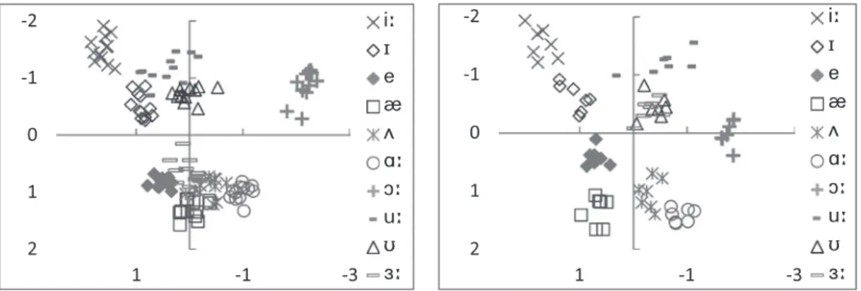
Figures 1 and 2 show the distribution of vowels produced by BN and AN, and Table 1 presents the results of their discriminant analyses. The normalized F2 mel values are represented on the x-axis and the normalized F1 mel values on the y-axis in the graphs. Each plot corresponds to the averaged F1/F2 mel value for a speaker. In Table 1, the percent at which the tokens were classified into the vowel category they intended (indicated by underlines) and into another category is reported. The numerals outside of and within the square brackets refer to the rates of BN and AN respectively. It should be also noted some values do not add up to 100% because they are rounded off to the nearest whole number.
The overall correct classification rate was 92% for BN and 90% for AN. This indicates the native speak- ers discriminated the vowels relatively well using the F1/F2 parameters.
These results demonstrated both similarities and differences between BN and AN. The differences
Figure 1. BN’s Vowel Distribution Figure 2. AN’s Vowel Distribution
lay in the way of distributing the vowels, which quite likely resulted from each accent. The most striking difference was as far as Figures 1 and 2 are visually compared. AN’s sounded much higher and more back than BN’s, and unlike BN’s it was closely integrated with , which means F1/F2 param- eters did not clearly distinguish them from each other. This was probably caused by an intrusion of
into the category, because the former is always preceded by in American English as usually tran- scribed [ in this accent, whose anticipatory coarticulation of lip rounding could add a -like quality on . Other parameters such as F3 and duration possibly function more crucially to discriminate them. Other visually apparent differences were in . sounded lower, [ more back, more front and higher in BN than AN. British English has one more monophthong, the low back vowel , which probably pushed up .
In spite of these differences, it was obvious BN and AN were analogous in that most of the vowels formed their own category in the auditory space, with a sharp dividing line from the adjacent vowel(s).
As for BN, for instance, although crowded in one place more evidently than those produced by AN, each did not completely overlap and delicately maintained their own category in a very dense area. This was mostly supported by the results of the discriminant analysis, which showed BN classified 100% correctly and well-classified at the rate of 83%. Regarding , BN confused it with other vowels like more frequently than visually observed. The correct classifica- tion rate of 75% was not extremely low, but a little confusion inevitably arose because the vowels were densely located in this area. This also extended to . It was classified 75% correctly, and a slight confusion with and occurred. BN’s was located more front, and it may have caused this Table 1. Results of the Discriminant Analysis for BN and AN
Predicted category
100[100]
100[100]
100[100]
83[100] 17
8 83[100] 8
100[100]
100[100]
8 [14] 75[86] 17
100[57] [43]
17 8 [43] 75[57]
Note. For BN and AN, 8% and 14% are equal to 1 person respectively. The values were rounded to the nearest whole number.
confusion with the high vowels centrally located. In addition, because the lip rounding characteristic of this vowel is rather reflected in F3 parameter, if F3 had been counted, would have been distinct from the other vowels. The rest of the vowels were distributed less densely, and [ espe- cially became an independent category isolated from any other vowel. This was further proved by the discriminant analysis which yielded the results that these vowels were accurately classified at the rate of 100%.
Figure 2 displays that, as with BN, AN successfully established a very distinct vowel category, along with the results of the discriminant analysis. There were two exceptions, , as discussed above, but the other vowels were classified highly correctly. gained the correct classification rate of 100%, and was 86% correctly classified. Nishi et al. (2008) found confusion between
and , but this study did not. Without invasion of into , would have been well-classified as well. Also, AN’s boundaries between each category seemed more defined than BN’s as in Figures 1 and 2. For example, AN’s was more front than BN’s, which created room for AN’s to survive in this area more comfortably. A higher correct classification rate of in AN was probably attributed to this.
3.2 JL
A one-way ANOVA was performed to select the candidates of high JL and low JL and found a sig- nificant difference in the score of the structural difference among the groups when the top seven and bottom seven JL were chosen, F(3, 29) = 419.16, p < .001. A Turkey’s HSD test yielded no significant difference between the top seven JL and AN, categorizing them as homogenous subsets, while both differed significantly from BN and the bottom seven JL. Further analysis was done with 12 BN, 7 AN, 14 high JL and 14 low JL.
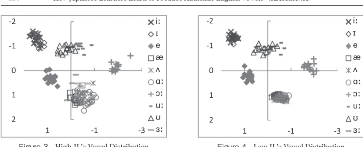
3.2.1 The distribution of F1/F2
Figures 3 and 4 present the distribution of vowels produced by high JL and low JL. This comparison will give a comprehensive picture of the developing process. These graphs display the underlying com- monality among JL: the five categories in the vowel space are easily recognizable, which were most likely founded on the Japanese five vowel categories. The results of the discriminant analysis for each group corroborated the existence of the five Japanese vowel categories as their base in learning English vowels. Compared to BN and AN, JL confused the vowels within specific vowels and almost always reciprocal confusion occurred within them. , and were paired or grouped and they were mutually confused within each pair or group, while and were never involved in these confusion matrices. This clearly shows that JL’s vowel space had five areas with well-defined borders.
However, high JL and low JL varied as well. Figures 3 and 4 show each of the areas of low JL espe- cially shrunk more than that of high JL, and they depict the sparseness of high JL and the denseness of low JL. In these areas, F1 mel values of high JL covered a wider range for all vowels. This was also reflected in the overall correct classification rate of 75% for high JL and 59% for low JL. In addition, this may not be outstanding enough, but high JL’s and seemed slightly more separated. These dif- ferences are associated with the development of L2 vowel learning.
3.2.2 The comparison of the vowel categories between high JL and low JL
The results of the discriminant analysis of high JL’s and low JL’s English vowels under the classifica- tion rules of BN and AN are summarized in Tables 2 and 3. The numerals outside of and within the square brackets represent the results of high JL and low JL respectively. The underlined percentages indicate the rates at which the tokens were classified into the model category the subjects intended. As a whole, 57% and 61% of the high JL’s tokens were each classified into BN and AN model categories, and 47% of the low JL’s tokens were in both.
A 4×2 mixed design ANOVA was also conducted in order to detect a significant difference among high JL, low JL, BN and AN, where the groups were a between-subject factor and the formant values were a within-subject factor. The results revealed a significant main effect of group for all the vowels but
and a significant interaction of formant and group for all the vowels, as represented in Table 4. As for the vowels which yielded the significant interaction effect, simple effects were further tested, and it was confirmed that there were significant simple main effects of group on F1/F2 mel values for all with two exceptions, an effect on F1 of [ and F2 of . Bonferroni pairwise comparisons (p < .05) were, then, carried out. The results will be discussed below, along with those of the discriminant analysis.
First, high JL and low JL showed a significant difference for , signaling high JL’s development in English vowel production. They differed in F1/F2 mel values of and F2 mel values of . For
Figure 4. Low JL’s Vowel Distribution Figure 3. High JL’s Vowel Distribution
, the results of the discriminant analysis supported this: 21% of high JL’s was classified into BN’s while no token of low JL was. A comparison to AN might make less sense because of its intru- sion to as discussed in 3.1, but the marginal superiority of high JL over low JL was revealed, too.
Clearly, the spread of their F1 mel values noted in 3.2.1 contributed to this superiority of high JL; there- fore, high JL resulted in no confusion with the low vowel and some confusion with the mid vowel
. However, high JL had not improved radically enough to form a new, complete category, considering Table 2: Results of the Discriminant Analysis of JL with BN as the Input Set
Predicted category
93[100] 7
86[100] 14
29[43] 71[57]
71 21[100] 7
29[7] 57[64] 14[29]
7 7[36] 86[64]
100[100]
[21] 100[79]
7[7] 36[29] 57[64]
7[64] 71[36] 21
Note. The rate is expressed in percentiles: 7% = 1 person. The values were rounded to the nearest whole number.
Table 3. Results of the Discriminant Analysis of JL with AN as the Input Set Predicted category
86[100] 14
57[100] 43
[7] 100[93]
100[100]
93[79] 7[21]
14[50] 86[50]
100[100]
[14] 93[50] 7[7] [28]
36[36] 43[43] 7 14[21]
93[71] [29] 7
Note. The rate is expressed in percentiles: 7% = 1 person. The values were rounded to the nearest whole number.
the majority of was still classified into others, such as . As for , although it is ongoing, a sig- nificant difference in F2 mel values of between high JL and low JL certainly proved high JL’s devel- opment toward establishing a new category. AN’s located quite front as drawn in Figure 2 laid down a strict condition on JL’s reaching AN’s level, but high JL sure approximated BN: 71% of the high JL’s tokens were classified into BN’s whereas 100% of low JL’s tokens were into BN’s . Taking into account BN themselves a little confused with , this rate can be regarded as fairly high. Besides, low JL, but not high JL, differed from BN at a significant level, which emphasized this result.
Second, there were some vowels which were not significantly different between high JL and low JL, but whose improvement in high JL was implied by the results of the discriminant analysis: and possibly . The reason why the difference did not reach a significant level varied from vowel to vowel. As for , high JL would not be sufficiently better. Both high JL’s and low JL’s differed sig- nificantly from BN’s and AN’s. However, 14% and 43% of high JL’s tokens were classified into BN’s and AN’s whilst none of low JL’s were. This suggests the category was in process of formation, but high JL’s was still located near low JL’s, far away from the natives.’ The finding in slightly dif- fered from that in in two respects. One was that high HL’s was classified into both BN’s and AN’s model category at the very high rate of 86%. The other was that low JL’s was also classified into BN’s and AN’s at a relatively high rate (64% and 50%). Therefore, no significant difference was found between high JL and low JL possibly due to a subtle ceiling effect. Also, the pairwise comparisons to BN and AN yielded a complex result that high JL’s F1 mel values and low JL’s F2 mel values were each significantly different from both BN’ and AN’s. High JL’s stretching of F1 mel values in the area mentioned in 3.2.1 might have unnecessarily changed their F1 mel values. However, high JL’s higher Table 4: Results of the 4×2 Mixed Design ANOVA
Main effect of group Formant × Group interaction
dfM dfR F p dfM dfR F p
3 43 0.18 .91 3 43 6.37 <.001
3 43 7.42 <.001 3 43 66.31 <.001
3 43 5.86 <.001 3 43 40.58 <.001
3 43 49.81 <.001 3 43 21.98 <.001
3 43 0.70 .56 3 43 9.13 <.001
3 43 10.39 <.001 3 43 10.30 <.001
3 43 34.81 <.001 3 43 12.46 <.001
3 43 10.11 <.001 3 43 16.86 <.001
3 43 6.21 <.001 3 43 11.86 <.001
3 43 39.36 <.001 3 43 70.53 <.001
classification rate into the model category proved their general development to encourage the formation of a more distinct category for . As for , it was comparable with in a good performance of low JL. The same or an even higher classification rate into BN’s and AN’s model category gained by low JL (64% and 79%) must have triggered a ceiling effect. In contrast, the difference from was that a mixed result was generated for in a comparison with BN and AN. High JL’s was classified into BN’s and AN’s at the rates of 57% and 93% respectively. It follows they almost completed forming
category if compared with AN, but they had not if compared with BN. The decrease from low JL’s 64% to high JL’s 57% could even mean a slight deterioration in high JL, but it is negligible too because this drop was equivalent to one subject’s error. Part of the reason for this can be that some tokens of high JL’s spread its category in the vowel space more than necessary, influenced by the improve- ment of . BN and AN placed a little differently although it barely stands out in Figures 1 and 2, and high JL’s still fell into AN’s model category successfully after being influenced by a change in other vowels, but it did not drop into BN’s. Nonetheless, the results of the pairwise comparisons found a significant difference only between low JL and AN. Thus, it would not be fair to argue high JL produced
less authentically. However, another problem is whether a closeness of JL’s to AN’s is acceptable.
JL’s , which shared a certain area in the vowel space with, approximated BN’s as discussed above. This led and which belonged to a different accent to coexist in one area, which may not be compatible. For , it would be better to adjust more to BN-like . The case in was much less straightforward. High JL’s and low JL’s were each classified into BN’s model category at the rates of 0% and 21% and into AN’s, at the rates of 93% and 50%. Seemingly, these results from the discriminant analysis provided the opposite results depending on the classification rule focused on, BN or AN. To put it simply, when focused on a comparison with BN, low JL performed better; when focused on that with AN, high JL did better. This was definitely attributed to the different distribution of
between BN and AN as pointed out in 3.1, which the pairwise comparisons found to be significant.
However, the classification rates of 21% and 50% that low JL reached were not high enough to claim this vowel category was completely formed in a very real sense. Rather, the category being created wan- dered somewhere between the BN and AN categories, perhaps a little closer to AN’s. On the contrary, 93% of high JL’s being classified into AN’s model category suggests high JL had created a category proper for around AN’s location. High JL’s closeness to AN was half proved by the results of the pairwise comparisons: whereas low JL’s F1/F2 mel values of were significantly different from BN’s and AN’s, only high JL’s F2 mel values were. A slight modification will be needed in the F2 mel values for high JL to be more native-like and gain a significant difference from low JL; however, almost 100%
correct classification into the model category should be regarded as the development of high JL.
Third, some vowels were apparently produced well by both low JL and high JL: . Because
they were successful in creating their own category from the very start for these vowels, no significant difference of the two groups was found certainly due to a ceiling effect. High JL and low JL also showed no significant difference in from AN and in from BN. Above all, 100% of both high JL and low JL classified into BN’s and AN’s , which suggests that JL easily produced . No other vowel being categorized into also proved its distinctiveness. Similarly, English was by no means prob- lematic for JL by AN standards since a very high percentage (100% and 93%) of high JL’s and low JL’s
were classified into AN’s and no other token was classified into it. The road to BN’s level would be a bit tougher because BN produced much lower , as described in 3.1, than JL’s , which was too high to prevent a little confusion with . However, a higher classification rate into BN’s model category for high JL (71%) than low JL (57%) evidenced the former’s approximation to BN to some extent.
requires a little more consideration. Low JL’s was 100% classified into the model category of BN and AN, which means JL have no problem establishing a category for this vowel. Nevertheless, high JL’s
gained a slightly lower correct classification rate. Though it was still high compared with other vowels, 7% and 14% of their tokens were each categorized into BN’s and AN’s . This could be due to high JL going the wrong way to form a distinct category in a sense, but another possible reason is that this was simply a side effect of the developing process, attributed to . From Figures 1, 2, 3 and 4, obviously JL’s was off the native location, sounding higher. reasonably occupied the Japanese category, so that high JL’s started forming a new category as mentioned above. However, and were still too alike for JL to distinguish in terms of their quality. With these two factors involved, high JL’s was slightly dragged to in the process of forming the category and some tokens were classified into
. Conversely, because low JL did not take action to form a new category for , their was consis- tently classified into the model category.
Finally, high JL’s and low JL’s indicated neither a significant difference nor high JL’s superiority in the classification rate into the model category. High JL was lower by 7% than low JL under both clas- sification rules although this one error made by one subject does not probably affect the overall trend as in . Figures 3 and 4 do not emphasize the difference in [ between high JL and low JL, either.
This does not, however, mean JL easily established the category as with . Their was classified into the model category less often, 57% and 64% at best under BN’s classification rule. Also, the results of the pairwise comparisons showed room for improvement: both high JL and low JL differed from BN and AN significantly in F1 mel values; low JL’s F2 mel values differed from AN. On the other hand, that JL’s was closer to BN’s than AN’s is a positive inclination. The same situation as
occurred with : BN-like and AN-like shared one area. However, these vowels were com- patible and did not lead to confusion because AN’s [ was located more back and BN’s was more front. Hence, this combination is not only practical but also safe.
3.3 General Discussion
The results of the present study showed that Japanese learners of English who had not specifically focused on pronunciation in their learning succeeded in discriminating some English vowels from others, or started to form new categories. Next, the results will be summarized and discussed, and the hypotheses in 1.5 will be also examined.
The vowels that supported the hypotheses included identical , new and similar . For , both high JL and low JL formed an authentic category successfully in the L2 vowel space. This proved to be identical to . Regarding , to set AN as a better reference for JL, high JL had formed a category and classified almost all tokens into the model category, but low JL had not. A very high classification rate for high JL indicates this vowel did not match the tendency of similar and new vowels, which validated the claim that was identical. However, the results imply was not as easy to use as the other identical vowel, . It turns out identical vowels vary in the speed of acquisition, unexpectedly. was confirmed to be forming a new category at least in a comparison with BN, and this strengthens the results of Lambacher et al. (2005) and Ingram and Park (1997). The two findings that high JL showed a far better performance than low JL and the category was better formed than other vowels categorized as similar demonstrate this vowel is neither identical nor similar, but new.
If they have formed their own category, their will sound more front. failed to testify it had a distinct category and did not provide an even faint hint of development from low JL to high JL. It leads to the conclusion that is similar to and forming a category is far from easy. also fulfilled the prediction that it was similar to , but lack of the monophthong which threatened ’s use of the
category led both high JL and low JL to produce fitting 100% into AN’s and BN’s model category.
No confusion, including with , might even suggest is identical to .
There were also vowels which did not partially uphold the hypothesis: . Based on Strange et al.
(1998) and Nishi et al. (2008), was categorized as similar, but confusion with decreased in high JL, especially under the classification rule of AN, and formed a distinct category uninterrupted by the other vowels. Accordingly, the prediction that Japanese would serve tentatively as the English
category was verified, but considering it was classified into AN’s model category at the rate of 100%, the categorization of into similar will invite questions.
For , further research on the learners at various L2 learning stages or in different learning environments is needed to prove the hypotheses. There was a significant difference in between low JL and high JL; however, the formation of the new category for this vowel was at a much earlier stage unlike . It has to be stably located higher. Therefore, insisting [ easily created its category is an hasty decision. A possible reason why this study did not reproduce the results of Lambacher et al.
(2005) is most likely because the subjects in their study were trained, but those in this study were not.
may be easy to form a category once learners know how to pronounce it authentically. As for , categorized as similar, it was supposed to fail in forming a new category according to the hypothesis;
however, high JL achieved a much better category than low JL, unlike another similar phone, . Nearly half of high JL’s tokens were classified into AN’s model category. This implies a possibility of the formation of the new category, which does not bear out the hypothesis. However, the correct classifica- tion rate into the model category was not high enough to conclude the category had been established.
has to be lower. Hence, the difficulty in forming this category remains unexplained.
As for the two undefined vowels , it is most reasonable to categorize as identical and
as similar or identical, suppose identical vowels allow for the slight difference in the speed of acquisi- tion as in . Unlike the other identical vowels, however, are identical to the length-dependent allophone, not phoneme. High JL classified into BN’s and AN’s model category fairly well. This sug- gests the category was easily formed the way the AN-like category was created for ; therefore, rea- sonably is identical to long . In contrast, high JL’s gained an even higher correct classifica- tion rate into the model category of AN, but not BN. This provides proof that BN’s is similar to short
whereas AN’s [ is identical to it. The former case is simple and enables the author to argue this is why had yet to establish its category and to be distinguished from and . The latter case is also acceptable. As suggested in the SLM, the similarity between L1 and L2 phones needs considering at an allophonic level although Flege (1995) limited allophones depending on position, strictly speaking. In addition, this finding is consistent with that of Nishi et al. (2008), where Japanese long and short
were mostly classified into American English and respectively. Thus, long and short
each fitted into AN’s and , and contributed to form distinct categories.
4. Conclusion
This study revealed that Japanese learners of English formed their English vowel categories without special emphasis being put on pronunciation in their learning, although how much they were completed differed from vowel to vowel. The vowels which needed more modification were no matter which norm learners set as their goal, British English or American English. Likewise, and
would allow improvement if learners aspire to acquire British English and American English respec- tively. As for the SLM, while it was mostly validated, there was room for further research into vowels like
. To test learners at various stages of English learning or in different learning environments will give a more robust answer to the question of how much the SLM predicts the learning of L2 segments.
Acknowledgements
This research made use of publicly available speech databases, the ULC Speaker Database and the
AUE Audio Archive. The author expresses her gratitude to the providers. Appreciation is also extended to her students for their participation in the experiment, Jonathan Harrison for his “anytime” help and Prof. Michiko Nakano for her innovative advice and uplifting comments.
References
Adank, P., Smits, R., & van Hout, R. (2004). A comparison of vowel normalization procedures for language variation research. Journal of the Acoustical Society of America, 116(5), 3099–3107.
Anderson-Hsieh, J., Johnson, R., & Koehler, K. (1992). The relationship between native speaker judgments of nonna- tive pronunciation and deviance in segmentals, prosody and syllable structure. Language Learning, 42(2), 529–
555.
Best, C. T. (1995). A direct realist view of cross-language speech perception. In W. Strange (Ed.), Speech perception and linguistic experience: Issues in cross-language research (pp. 171–204). Timonium, MD: York Press.
Derwing, T. M., & Rossiter, M. J. (2003). The effects of pronunciation instruction on the accuracy, fluency and com- plexity of L2 accented speech. Applied Language Learning, 13, 1–18.
Flege, J. E. (1987). The production of “new” and “similar” phones in a foreign language: evidence for the effect of equivalence classification. Journal of Phonetics, 15, 47–65.
Flege, J. E. (1995). Second language speech learning: Theory, findings, and problems. In W. Strange (Ed.), Speech perception and linguistic experience: Issues in cross-language research (pp. 233–277). Timonium, MD: York Press.
Ingram, J. C. L., & Park, S. (1997). Cross-language vowel perception and production by Japanese and Korean learners of English. Journal of Phonetics, 25, 343–370.
Jenkins, J. (2000). The phonology of English as an international language. Oxford: Oxford University Press.
Kuhl, P. K. (2000). A new view of language acquisition. Proceedings of the National Academy of Sciences, USA, 97, 11850–11857.
Ladefoged, P. (2003). Phonetic data Analysis: A introduction to Fieldwork and Instrumental Techniques. Malden, MA:
Blackwell.
Lambacher, S. G., Martens, W. L., Kakehi, K., Marasinghe, C. A., & Molholt, G. (2005). The effects of identification training on the identification and production of American English vowels by native speakers of Japanese. Applied Psycholinguistics, 26, 227–247.
Lobanov, B. M. (1971). Classification of Russian Vowels Spoken by Different Speakers. Journal of the Acoustical Society of America, 49, 606–608.
Markham, D., & Hazan, V. (2002). The UCL speaker database. Speech, Hearing and Language: UCL Work in Progress, 14, 1–17.
Merfert, I. (1997). The alt.usage.english Audio Archive. Retrieved from http://alt-usage-english.org/index.shtml Nishi, K., Strange, W., Akahane-Yamada, R., Kubo, R., & Trent-Brown, S. A. (2008). Acoustic and perceptual similarity
of Japanese and American English vowels. Journal of the Acoustical Society of America, 124(1), 576–588.
Strange, W., Akahane-Yamada, R., Kubo, R., Trent, S. A., Nishi, K., & Jenkins, J. J. (1998). Perceptual assimilation of American English vowels by Japanese listeners. Journal of Phonetics, 26, 311–344.
Strange, W., Weber, A., Levy, E. S., Shafiro, V., Higashi, M., & Nishi, K. (2007). Acoustic variability within and across German, French, and American English vowels: Phonetic context effects. Journal of the Acoustical Society of America, 122(2), 1111–1129.
Suzuki, M., Qiao, Y., Minematsu, N., & Hirose, K. (2010). Integration of multilayer regression analysis with structure- based pronunciation assessment. INTERSPEECH 2010, 586–589.
Tsujimura, N. (2006). An introduction to Japanese linguistics (2nd ed.). Malden, MA: Blackwell.
ABSTRACT
How Japanese Learners Learn to Produce Authentic English Vowels Aya Kitagawa
This study investigated the pronunciation of English vowels produced by Japanese learners who had not specifically focused on pronunciation in their learning. In order to examine the learning process within the framework of the speech learning model (SLM), Japanese learners with high and low profi- ciency in English were compared with native speakers of British English and American English in the production of English monophthongs. As a result, it was discovered Japanese learners learned to pro- duce successfully in the sense that these vowels were differentiated from others with quality. This generally sustained the formulated hypotheses based on the SLM.
![Table 3. Results of the Discriminant Analysis of JL with AN as the Input Set Predicted category 86[100] 14 57[100] 43 [7] 100[93] 100[100] 93[79] 7[21] 14[50] 86[50] 100[100] [14] 93[50] 7[7] [28] 36[36] 43[4](https://thumb-ap.123doks.com/thumbv2/123deta/9800760.1881989/11.773.85.685.140.404/table-results-discriminant-analysis-input-set-predicted-category.webp)
