c 2006. Astronomical Society of Japan.
Reliability Checks on the Indo-US Stellar Spectral Library Using Artificial Neural Networks and Principal Component Analysis
Harinder P. SINGH
Department of Physics and Astrophysics, University of Delhi, Delhi 110007, India [email protected]
Manabu YUASAand Nawo YAMAMOTO
Research Institute for Science and Technology, Kinki University, Higashi-Osaka, Osaka 577-8502 [email protected]
and Ranjan GUPTA
Inter-University Center for Astronomy and Astrophysics, Ganeshkhind, Pune 411007, India [email protected]
(Received 2005 October 21; accepted 2005 December 16) Abstract
The Indo-US coud´e feed stellar spectral library (CFLIB) made available to the astronomical community recently by Valdes et al. (2004, ApJS, 152, 251) contains spectra of 1273 stars in the spectral region 3460 to 9464 ˚A at a high resolution of 1 ˚A (FWHM) and a wide range of spectral types. Cross-checking the reliability of this database is an important and desirable exercise since a number of stars in this database have no known spectral types and a considerable fraction of stars has not so complete coverage in the full wavelength region of 3460–9464 ˚A resulting in gaps ranging from a few ˚A to several tens of ˚A. We use an automated classification scheme based on Artificial Neural Networks (ANN) to classify all 1273 stars in the database. In addition, principal component analysis (PCA) is carried out to reduce the dimensionality of the data set before the spectra are classified by the ANN. Most importantly, we have successfully demonstrated employment of a variation of the PCA technique to restore the missing data in a sample of 300 stars out of the CFLIB.
Key words:catalogs — methods: data analysis — stars: general 1. Introduction
Automated schemes of data validation and analysis have assumed added significance recently as larger databases are increasingly becoming available in almost all areas of obser- vational astronomy. With the advent of bigger CCD detectors in spectroscopy, the need for having large libraries of stellar spectra at high spectral resolution is also getting fulfilled.
Jacoby, Hunter, and Christian (1984, hereafter JHC) made 158 spectra available in the range of 3510–7427 ˚A at 4.5 ˚A resolution. Prugniel and Soubiran (2001) published a library of 708 stars using the ELODIE eschelle spectrograph at the Observatoire de Haute-Province that covers a wavelength band of 4100–6800 ˚A at a resolution ofR= 42000. Cenarro et al.
(2001) have provided a database of 706 stellar spectra in the wavelength region 8350–9020 ˚A at 1.5 ˚A resolution and Le Borgne et al. (2003, hereafter STELIB) with 247 spectra in the range of 3200–9500 ˚A at 3 ˚A resolution. Moultaka et al.
(2004, hereafter ELODIE) compiled 1959 spectra in the range of 4000–6800 ˚A at a resolution of 0.55 ˚A.
More recently, Valdes et al. (2004) observed more than 1200 stars with emphasis on broad wavelength coverage (3400–
9500 ˚A) at a resolution of∼1 ˚A (FWHM) at an original disper- sion of 0.44 ˚A per pixel. Their coud´e feed stellar spectral library (CFLIB) provides a resolution sufficient to resolve numerous diagnostic spectral features that can be used in the automated parameterization of spectra.
Neural networks are a form of multiprocessor computing system, with simple processing elements with a high degree of inter-connection, simple scalar messaging, and adaptive inter- action between elements. In a supervised back propagation algorithm, the network topology is constrained to be feed- forward, i.e., connections are generally allowed from the input layer to the first (and mostly only) hidden layer; from the first hidden layer to the second, . . . , and from the last hidden layer to the output layer. The hidden layer learns to recode (or to provide a representation for) the inputs. More than one hidden layer can be used. The architecture is more powerful than single-layer networks: it can be shown that any mapping can be learned, given two hidden layers (of units).
Automated schemes like the Artificial Neural Networks (ANN) have been used in Astronomy for a number of data analysis tasks like scheduling observations (Johnston, Adorf 1992), adaptive optics (Angel et al. 1990), stellar spectral classification (Gulati et al. 1994; von Hippel et al. 1994), and star–galaxy separation studies (Odewahn et al. 1992). In addition Gulati, Gupta, and Rao (1997a) extended the ANN analysis to compare synthetic and observed spectra of G and K dwarfs. Gulati, Gupta, and Singh (1997b) estimated inter- stellar extinctionE(B−V) using ANN from low-dispersion ultraviolet spectra for O and B stars. Bailer-Jones, Gupta, and Singh (2002) provide a review of the ANN applications in astronomical spectroscopy.
Another powerful statistical tool for data analysis is the
178 H. P. Singh et al. [Vol. 58,
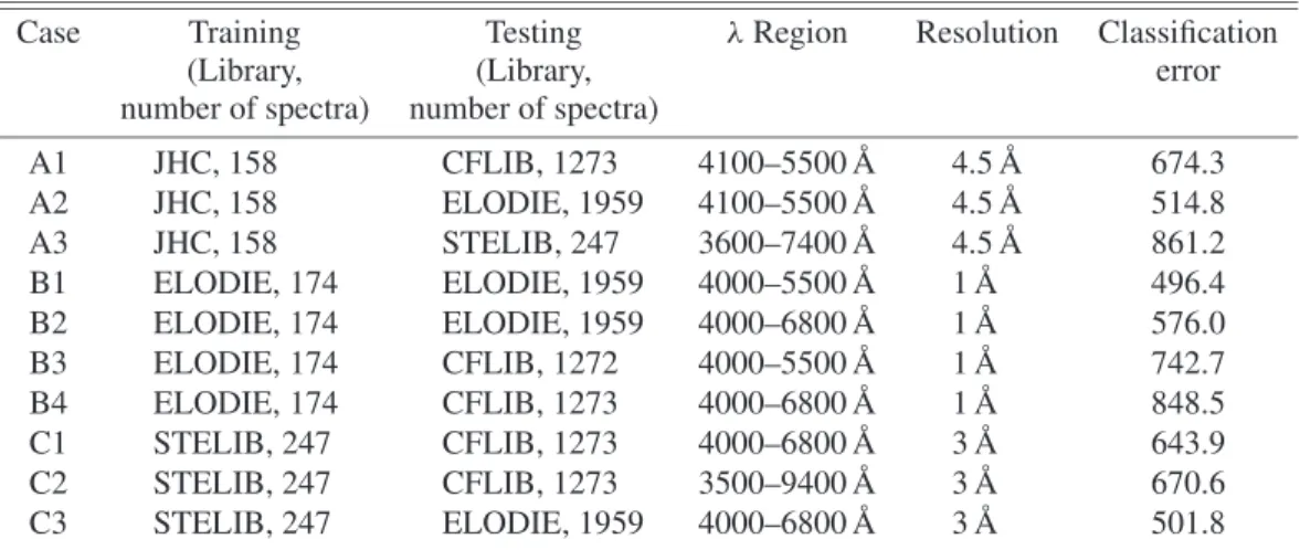
Table 1. ANN training and test cases.∗
Case Training Testing λRegion Resolution Classification
(Library, (Library, error
number of spectra) number of spectra)
A1 JHC, 158 CFLIB, 1273 4100–5500 ˚A 4.5 ˚A 674.3
A2 JHC, 158 ELODIE, 1959 4100–5500 ˚A 4.5 ˚A 514.8
A3 JHC, 158 STELIB, 247 3600–7400 ˚A 4.5 ˚A 861.2
B1 ELODIE, 174 ELODIE, 1959 4000–5500 ˚A 1 ˚A 496.4
B2 ELODIE, 174 ELODIE, 1959 4000–6800 ˚A 1 ˚A 576.0
B3 ELODIE, 174 CFLIB, 1272 4000–5500 ˚A 1 ˚A 742.7
B4 ELODIE, 174 CFLIB, 1273 4000–6800 ˚A 1 ˚A 848.5
C1 STELIB, 247 CFLIB, 1273 4000–6800 ˚A 3 ˚A 643.9
C2 STELIB, 247 CFLIB, 1273 3500–9400 ˚A 3 ˚A 670.6
C3 STELIB, 247 ELODIE, 1959 4000–6800 ˚A 3 ˚A 501.8
∗Two hidden layers were used for all the cases.
principal component analysis (PCA). It involves a mathe- matical procedure that transforms a number of (possibly) correlated variables into a (smaller) number of uncorrelated variables called principal components. The first principal component accounts for as much of the variability in the data as possible, and each succeeding component accounts for as much of the remaining variability as possible. Objectives of principal component analysis are to discover or to reduce the dimensionality of a data set and to identify new meaningful underlying variables. The technique has been used widely for a number of applications in Astronomy, viz., for stellar classi- fication by Murtagh and Heck (1987), Storrie-Lombardi et al.
(1994), and Singh et al. (1998), by Francis et al. (1992) for QSO spectra, and for galaxy spectra by Sodr´e and Cuevas (1994), Connolly et al. (1995), Lahav et al. (1996), and Folkes, Lahav, and Maddox (1996).
Another important application was developed by Unno and Yuasa (1992, 2000) for supplementing missing observational data using a generalized PCA technique. Subsequently, Yuasa, Unno, and Magono (1999) made use of this technique to deter- mine distances of 183 mass-losing red giants.
The primary aim of this paper is to perform validity checks on the CFLIB by running the ANN code on various inter library sets like JHC, ELODIE, and STELIB. In the next section we describe the ANN analysis. In section 3, we demonstrate the possibility of using PCA for filling the gaps in the spectra of CFLIB. In section 4, we summarize important conclusions of the study.
2. ANN Analysis
A classification scheme using ANN involves two stages: a training stage and a testing stage. In the training stage, the input patterns and the desired output patterns are defined before the learning process of the ANN is carried out. During training, the network output and the desired output are compared and the network weights are adjusted. We employ a back propa- gation algorithm (Rumelhart et al. 1986) to achieve this. The learning is stopped when the desired error threshold is reached
and the network weights are frozen for use with the test set. In the testing stage, the test patterns are used by the network and classified in terms of the training classes.
In what follows, we have trained the ANN on three libraries with a view to run validity checks on the CFLIB. Three libraries that we used for training are:
1. JHC (Jacoby et al. 1984) with 158 spectra available in the range of 3510–7427 ˚A at 4.5 ˚A resolution
2. ELODIE (Moultaka et al. 2004) with 1959 spectra in the range of 4000–6800 ˚A at a resolution of 0.55 ˚A
3. STELIB (Le Borgne et al. 2003) with 247 spectra in the range of 3200–9500 ˚A at 3 ˚A resolution
A total of 10 test cases were run and are summarized in table 1. We also give the wavelength region used in each case, resolution, and the resulting classification error. Cases A1–A3 involved training of the ANN by JHC and testing on, respec- tively, the CFLIB, ELODIE, and STELIB. Cases B1–B4 involved training the ANN with 174 individual classes of ELODIE and testing on ELODIE (4000–5500 ˚A, Case B1), ELODIE (4000–6800 ˚A, Case B2), CFLIB (4000–5500 ˚A, Case B3), and CFLIB (4000–6800 ˚A, Case B4). The last three cases C1–C3 involved training on STELIB and testing on CFLIB (4000–6800 ˚A, Case C1), CFLIB (3500–9400 ˚A, Case C2), and ELODIE (4000–6800 ˚A, Case C3).
The resolution used for training and testing for cases A1–A3 is 4.5 ˚A which is the resolution of JHC, 1 ˚A for cases B1–B4 which is the resolution of CFLIB, and 3 ˚A for cases C1–C3 which is the resolution of STELIB. The higher resolutions of some of the testing cases were degraded to match the resolution of the training library by Gaussian convolution. The testing is done on the complete libraries, i.e., for 247 stars of STELIB, 1959 stars of ELODIE, and 1273 stars of CFLIB.
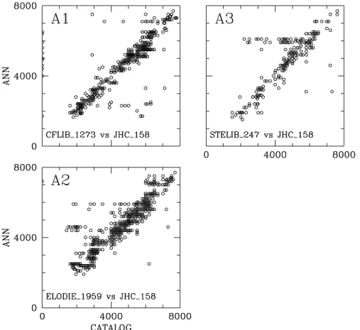
The classification scatter plots from these analyses are shown in figures 1–3. The MK spectral types have been coded numerically for use by the ANN. The MK alphabetic type O is given a numeric code of 1000, B is 2000, A is 3000, and so on with M being 7000. The subclasses are multiplied by 100 and added in, thus an F5 star is coded as 4500. The luminosity
Fig. 1. Classification scatter plots for Cases A1–A3. Expression by numbers in axes for classification is referred to the text.
Fig. 2. Classification scatter plots for Case B1–B4.
180 H. P. Singh et al. [Vol. 58,
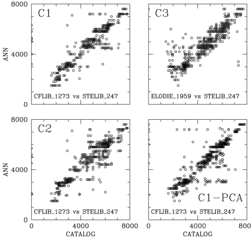
Fig. 3. Classification scatter plots for Case C1–C3. Also shown is case C1 with PCA preprocessing where first 15 principal components were used.
classes I, II, III, IV, and V are coded as 1.5, 3.5, 5.5, 7.5, and 9.5, respectively. An F5 V star is thus coded as 4509.5. In the present scheme, the luminosity class is given a low weight and the main emphasis on classification of the spectral types.
In the following we provide a discussion on the classification accuracy of the three sets of cases:
Cases A1–A3
The Cases A1–A3 use JHC as the training set with A1 and A2 in the wavelength region 4100–5500 ˚A, i.e., in the blue part of the spectrum. In the case A3, JHC was trained for the full span i.e. 3600–7400 ˚A and tested on STELIB in the same band.
The blue region classification error is lowest for ELODIE and somewhat inferior for CFLIB. However, the full span classifi- cation of STELIB deteriorates the error to about 861, i.e., 8.6 sub-spectral-type.
Cases B1–B4
In Case B1–B4, ELODIE was used as the training set and was tested on both ELODIE and CFLIB in the blue and full span. The training set of 174 spectra was preselected from amongst the 1959 ELODIE full set with one example spectra per spectro–luminosity class. The best classification is obtained for the case B1 with blue region of ELODIE. For the same region of CFLIB, i.e., case B2, the classification is somewhat inferior. The full span classification case B3 for ELODIE and case B4 for CFLIB are consequently with higher classification errors.
Cases C1–C3
Cases C1–C3 use STELIB as the training set and the test sets are CFLIB limited span C1, ELODIE limited span C3, and CFLIB full span case C2. The limited span cases of C1 and C3 show errors of 6.43 and 5.01 sub-spectral types but remarkably the case C2 with full span shows an error of only 6.7.
The most useful result as far as CFLIB is concerned, is the case C2 since the largest wavelength span is used for this case.
It may be noted that except JHC, all other spectral libraries have gaps in them and this contributes greatly into the classifi- cation errors. Further, we also used a PCA based preprocessor for all the cases to reduce the dimensionality of the train–test sets as described in Singh et al. (1998). The resulting classi- fication errors using first 15 principal components are only marginally poorer than the ones listed in the last column of table 1. Last panel in figure 3 shows the scatter plot of case C1 with PCA.
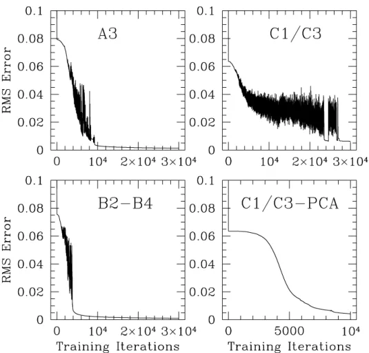
Figure 4 displays some example learning curves of the ANN training sessions for Cases A3, B2–B4, C1–C3, and a PCA version of C1–C3. The B2–B4 (and C1–C3) are same training sessions. All the learning curves fall to a low rms learning error at the level on number of iterations of 30000. The PCA version however requires much less number on iterations (∼10000) to bring down these errors.
Fig. 4. ANN training session learning curves for some selected cases.
3. Restoration of Missing Data Using PCA
To fill the gaps in the spectra one can use the data from a similar type star which doesn’t have a gap at the same wavelength. However, we present here a preliminary study of an automated method for restoration of missing data for a set of spectra of 300 stars in the wavelength region 4000–4300 ˚A selected from the CFLIB. The list of stars with their spectral types is given in table 3 in Appendix. The method of restora- tion is adopted from Unno and Yuasa (1992) and is briefly described here for the present data set.
To begin with, we have 301 flux values at 1 ˚A interval in the range for 4000–4300 ˚A for 300 stars. A sample of seven spectra are shown in figure 5. For thei-th star, letFjiandwji be thej-th observed flux value and its weight respectively, where j= 1,...,n(n= 301) andi= 1,...,N(N= 300). If a particular flux valueFjifor a particular star is missing, its weight is equal to zero.
For applying the PCA, the normalized datafji is defined as fji=
Fji− Fj
σj , (1)
whereFjandσj are the mean and the standard deviation of Fj respectively and are given by
Fig. 5. Representative spectra of seven stars out of the total of 300 stars. The spectral types are listed on the vertical axis.
182 H. P. Singh et al. [Vol. 58,
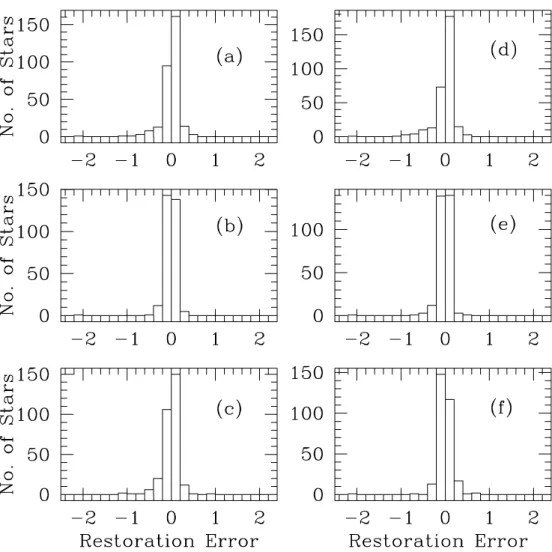
Fig. 6. Histogram of restoration error and the number of stars for the six cases. All stars with restoration errors greater than±0.2 are binned together.
Fj= N
i=1
wijFji N
i=1
wij
, (2)
and
σj2= N
i=1
wji
Fji− Fj2
N i=1
wij
. (3)
Following Unno and Yuasa (1992), we define virtual dataxij and their corresponding weightvijfor each observed flux value fjifor each star as
vij= 1−wji, (4)
N i=1
vijxji= 0, N
i=1
vij(xji)2= N
i=1
vji. (5)
Equation (5) represents the statistical constraint that the mean value of the virtual data is zero and the standard deviation is unity. For such a case, the correlation coefficient between the j-th quantity and thek-th quantity is defined by
Cjk= 1 N
N i=1
(wjifji +vijxji)(wikfki +vkixki). (6) The most probable value ofxji are thus given by the following set ofnsimultaneous linear algebraic equations:
n l=1
1 λl
µ2ljxji +
k=j
µljµlk(wikfki +vkixik)
= 0, (7) (j = 1,...,n),
where λl is the l-th eigenvalue and µjl represent the j-th component of the l-th eigenvector in the PCA. The final adjusted value for the normalizedj-th flux value for thei-th star is given by
wijfji +vjixji. (8) To check the veracity of this procedure let us assume that from the data set only one flux valueF1sis missing. This means
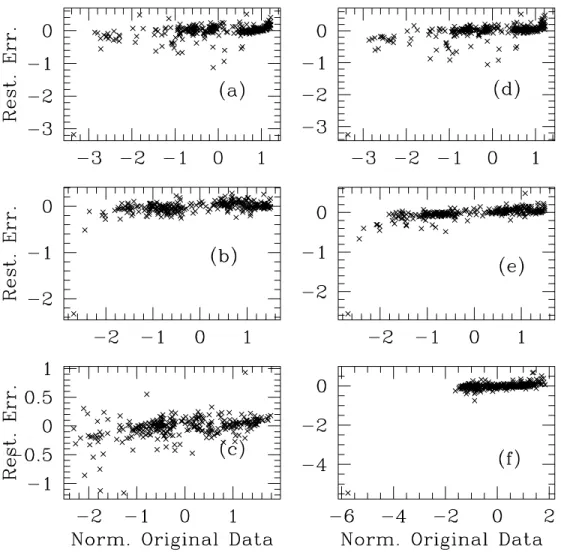
Fig. 7. Restoration error plotted against the normalized original data for all the six cases. The outlier at the bottom left of most of the plots is HD 31996.
Table 2. Cases studied for flux restoration analysis using PCA.
Case Reconstructed flux Number of principal components λregion
(a) 4000 ˚A 10 4000–4009 ˚A
(b) 4077 ˚A 10 4077–4086 ˚A
(c) 4291 ˚A 10 4291–4300 ˚A
(d) 4000 ˚A 20 4000–4019 ˚A
(e) 4077 ˚A 20 4077–4096 ˚A
(f) 4281 ˚A 20 4281–4300 ˚A
thatws1= 0 and all the other weightswji exceptws1are equal to unity. In this simplified situation, equations (7) reduce to
n
l=1
µ2l1
λl x1s + n
l=1
µl1
λl n
k=2
µlkfks = 0, (9) (s= 1,...,N).
Equation (9) can be easily solved to get x1s for the missing fluxf1s. By exchanging the columns, one can computex2s,x3s, and so on for the missing flux for any wavelength and for any
star. Six separate cases were studied and are listed in table 2.
The results of our preliminary analysis are shown in figures 6 and 7.
Case (a) uses a flux region of 10 ˚A starting from 4000 ˚A and thus 10 principal components to reconstruct the fluxes at 4000 ˚A for all the 300 stars. From figure 6a we see that 256 stars have restoration error (f1i−x1i) within±0.1. Figure 7a shows the restored error vs. original value of the normalized fluxf1i(with mean zero). It is clear that for most of the stars the reconstruction is good. Case (d) uses 20 principal components
184 H. P. Singh et al. [Vol. 58, and the reconstruction of flux at 4000 ˚A is comparable, maybe
slightly worse as is clear from figure 6d and figure 7d.
We also tested the validity of this flux reconstruction method by attempting to reproduce a strong absorption feature, namely the 4077 ˚A SrIIfeature, visible in the representative spectra in figure 5. Case (b) attempts to achieve this using 10 principal components rather successfully as is clear from figure 6b and figure 7b respectively. The flux at 4077 ˚A was reconstructed to within±0.1 for a total of 281 stars out of 300. The case (e) with 20 principal components also reproduces the flux at 4077 ˚A well although no better than case (b) (279 stars within±0.1) suggesting that the 10 PC’s are enough for the data reconstruc- tion in this data set. Lastly, cases (c) and (f) show similar behavior in reconstructing towards the end of the wavelength interval and the results are plotted in figure 6c and f, and figure 7c and f.
Another interesting offshoot of this analysis was in picking outliers, stars which have either no known MK spectral types or have noisy spectra. Figure 7a,b,d,e,f clearly show one outlier for which our scheme is unable to restore or reconstruct the fluxes. The star is HD 31996 and it indeed has no MK spectral class assigned to it (table 3) as was verified from the CFLIB and the SIMBAD database. Another star, HD 46687, also has no known spectral type but its spectrum resembles an M type star.
For this star, our analysis was able to reconstruct the fluxes.
The spectra of these two stars obtained from the CFLIB are plotted in figure 8.
4. Conclusions
We have performed an extensive analysis based on artificial neural networks to classify stars in an automated manner in the Indo-US CFLIB using three databases viz., JHC, STELIB, and ELODIE. The main aim of this exercise was two-fold. One was to perform the reliability checks on CFLIB to see how the gaps in the library affect the classification accuracy. We find that the despite the presence of gaps, we have achieved classification accuracy of less than one main class. The second aim was to evolve and test automated procedures of classifying stellar spectra. This was achieved by trying our ANN scheme on ten different cases of training and testing on different pairs of libraries. The schemes are numerically intensive, with the ANN training stage requiring several hours of CPU time on the fastest of workstations. A PCA analysis was employed successfully to reduce the dimensionality of the data set and hence faster training without appreciable loss in classification accuracy.
Both STELIB and ELODIE libraries have variable spans of wavelength gaps where the fluxes are filled with zeros (similar to CFLIB). Such gaps lead to classification errors in the PCA and ANN schemes. However, we have carried out some preliminary analysis with the basicχ2minimization scheme on
Fig. 8. Spectrum of the two stars HD 31996 and HD 46687 which have no known spectral types. Star HD 31996 is the outlier in the flux restoration analysis.
these libraries wherein the gap portions were omitted in both train and test sets. This lead to a remarkable improvements in the classification accuracy.
We have also employed a generalized principal component analysis to first create and then fill the gaps in a sample of 300 stars out of the CFLIB in the blue region. At present, we have used a simplified system to reconstruct flux values at one wavelength bin at a time for these 300 stars. We hope to exploit the full potential of the scheme and attempt to fill larger gaps in stellar spectra in a subsequent study.
MY and HPS are grateful to JSPS (Japan Society for Promotion of Science) and DST (Department of Science &
Technology, India) for financial support for exchange visits which made this work possible. MY would like to thank Emeritus Professor W. Unno of the University of Tokyo for helpful discussions. The research has made use of the SIMBAD database, operated by CDS, Strasbourg, France and the INDO-US CFLIB managed by NOAO, Tucson, AZ, USA.
Appendix. List of Stars for Data Restoration Analysis The list of 300 stars with their HD numbers and the spectral types is given in table 3. Two stars HD 31996 and HD 46687 have no known spectral types.
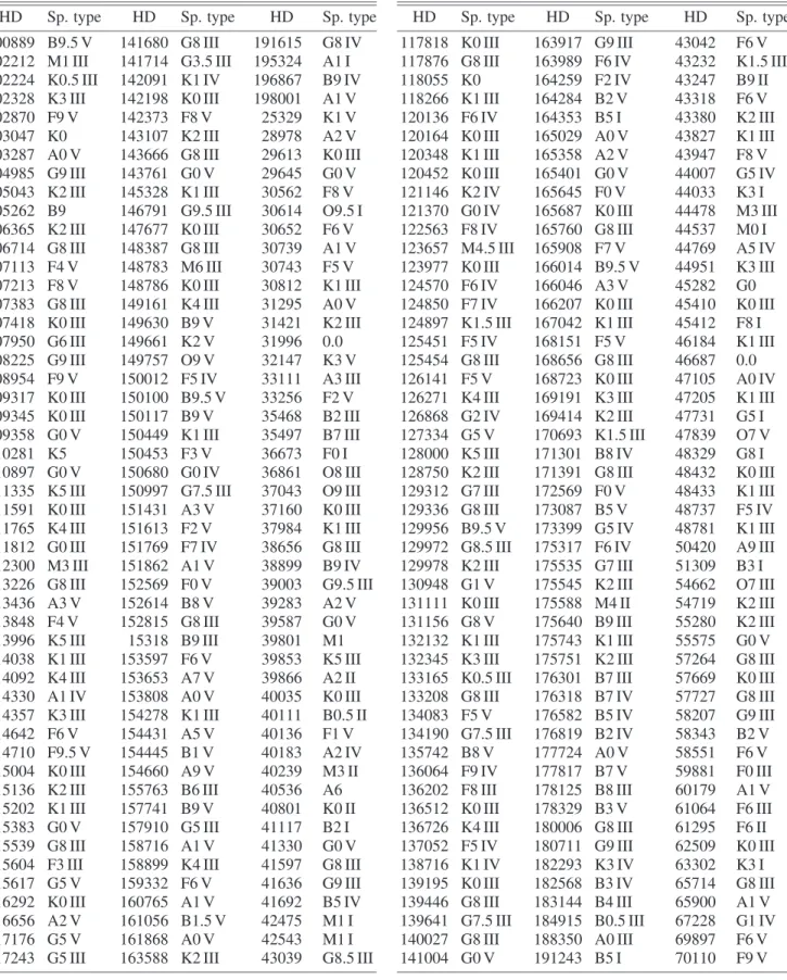
Table 3. Sample of 300 stars used for data restoration analysis.
HD Sp. type HD Sp. type HD Sp. type
100889 B9.5 V 141680 G8 III 191615 G8 IV 102212 M1 III 141714 G3.5 III 195324 A1 I 102224 K0.5 III 142091 K1 IV 196867 B9 IV 102328 K3 III 142198 K0 III 198001 A1 V
102870 F9 V 142373 F8 V 25329 K1 V
103047 K0 143107 K2 III 28978 A2 V
103287 A0 V 143666 G8 III 29613 K0 III 104985 G9 III 143761 G0 V 29645 G0 V 105043 K2 III 145328 K1 III 30562 F8 V 105262 B9 146791 G9.5 III 30614 O9.5 I 106365 K2 III 147677 K0 III 30652 F6 V 106714 G8 III 148387 G8 III 30739 A1 V 107113 F4 V 148783 M6 III 30743 F5 V 107213 F8 V 148786 K0 III 30812 K1 III 107383 G8 III 149161 K4 III 31295 A0 V 107418 K0 III 149630 B9 V 31421 K2 III 107950 G6 III 149661 K2 V 31996 0.0 108225 G9 III 149757 O9 V 32147 K3 V 108954 F9 V 150012 F5 IV 33111 A3 III 109317 K0 III 150100 B9.5 V 33256 F2 V 109345 K0 III 150117 B9 V 35468 B2 III 109358 G0 V 150449 K1 III 35497 B7 III
110281 K5 150453 F3 V 36673 F0 I
110897 G0 V 150680 G0 IV 36861 O8 III 111335 K5 III 150997 G7.5 III 37043 O9 III 111591 K0 III 151431 A3 V 37160 K0 III 111765 K4 III 151613 F2 V 37984 K1 III 111812 G0 III 151769 F7 IV 38656 G8 III 112300 M3 III 151862 A1 V 38899 B9 IV 113226 G8 III 152569 F0 V 39003 G9.5 III
113436 A3 V 152614 B8 V 39283 A2 V
113848 F4 V 152815 G8 III 39587 G0 V 113996 K5 III 15318 B9 III 39801 M1 114038 K1 III 153597 F6 V 39853 K5 III 114092 K4 III 153653 A7 V 39866 A2 II 114330 A1 IV 153808 A0 V 40035 K0 III 114357 K3 III 154278 K1 III 40111 B0.5 II 114642 F6 V 154431 A5 V 40136 F1 V 114710 F9.5 V 154445 B1 V 40183 A2 IV 115004 K0 III 154660 A9 V 40239 M3 II 115136 K2 III 155763 B6 III 40536 A6 115202 K1 III 157741 B9 V 40801 K0 II 115383 G0 V 157910 G5 III 41117 B2 I 115539 G8 III 158716 A1 V 41330 G0 V 115604 F3 III 158899 K4 III 41597 G8 III 115617 G5 V 159332 F6 V 41636 G9 III 116292 K0 III 160765 A1 V 41692 B5 IV 116656 A2 V 161056 B1.5 V 42475 M1 I 117176 G5 V 161868 A0 V 42543 M1 I 117243 G5 III 163588 K2 III 43039 G8.5 III
HD Sp. type HD Sp. type HD Sp. type
117818 K0 III 163917 G9 III 43042 F6 V 117876 G8 III 163989 F6 IV 43232 K1.5 III
118055 K0 164259 F2 IV 43247 B9 II
118266 K1 III 164284 B2 V 43318 F6 V 120136 F6 IV 164353 B5 I 43380 K2 III 120164 K0 III 165029 A0 V 43827 K1 III 120348 K1 III 165358 A2 V 43947 F8 V 120452 K0 III 165401 G0 V 44007 G5 IV 121146 K2 IV 165645 F0 V 44033 K3 I 121370 G0 IV 165687 K0 III 44478 M3 III 122563 F8 IV 165760 G8 III 44537 M0 I 123657 M4.5 III 165908 F7 V 44769 A5 IV 123977 K0 III 166014 B9.5 V 44951 K3 III
124570 F6 IV 166046 A3 V 45282 G0
124850 F7 IV 166207 K0 III 45410 K0 III 124897 K1.5 III 167042 K1 III 45412 F8 I 125451 F5 IV 168151 F5 V 46184 K1 III 125454 G8 III 168656 G8 III 46687 0.0 126141 F5 V 168723 K0 III 47105 A0 IV 126271 K4 III 169191 K3 III 47205 K1 III 126868 G2 IV 169414 K2 III 47731 G5 I 127334 G5 V 170693 K1.5 III 47839 O7 V 128000 K5 III 171301 B8 IV 48329 G8 I 128750 K2 III 171391 G8 III 48432 K0 III 129312 G7 III 172569 F0 V 48433 K1 III 129336 G8 III 173087 B5 V 48737 F5 IV 129956 B9.5 V 173399 G5 IV 48781 K1 III 129972 G8.5 III 175317 F6 IV 50420 A9 III 129978 K2 III 175535 G7 III 51309 B3 I 130948 G1 V 175545 K2 III 54662 O7 III 131111 K0 III 175588 M4 II 54719 K2 III 131156 G8 V 175640 B9 III 55280 K2 III 132132 K1 III 175743 K1 III 55575 G0 V 132345 K3 III 175751 K2 III 57264 G8 III 133165 K0.5 III 176301 B7 III 57669 K0 III 133208 G8 III 176318 B7 IV 57727 G8 III 134083 F5 V 176582 B5 IV 58207 G9 III 134190 G7.5 III 176819 B2 IV 58343 B2 V 135742 B8 V 177724 A0 V 58551 F6 V 136064 F9 IV 177817 B7 V 59881 F0 III 136202 F8 III 178125 B8 III 60179 A1 V 136512 K0 III 178329 B3 V 61064 F6 III 136726 K4 III 180006 G8 III 61295 F6 II 137052 F5 IV 180711 G9 III 62509 K0 III 138716 K1 IV 182293 K3 IV 63302 K3 I 139195 K0 III 182568 B3 IV 65714 G8 III 139446 G8 III 183144 B4 III 65900 A1 V 139641 G7.5 III 184915 B0.5 III 67228 G1 IV 140027 G8 III 188350 A0 III 69897 F6 V 141004 G0 V 191243 B5 I 70110 F9 V
186 H. P. Singh et al.
References
Angel, J. R. P., Wizinowich, P., Lloyd-Hart, M., & Sandler, D. 1990, Nature, 348, 221
Bailer-Jones, C. A. L., Gupta, R., & Singh, H. P. 2002, in Automated Data Analysis in Astronomy, ed. R. Gupta, H. P. Singh, & C. A. L.
Bailer-Jones (New Delhi: Narosa), 51
Cenarro, A. J., Cardiel, N., Gorgas, J., Peletier, R. F., Vazdekis, A., &
Prada, F. 2001, MNRAS, 326, 959
Connolly, A. J., Szalay, A. S., Bershady, M. A., Kinney, A. L., &
Calzetti, D. 1995, AJ, 110, 1071
Folkes, S. R., Lahav, O., & Maddox, S. J. 1996, MNRAS, 283, 651 Francis, P. J., Hewett, P. C., Foltz, C. B., & Chaffee, F. H. 1992, ApJ,
398, 476
Gulati, R. K., Gupta, R., Gothoskar, P., & Khobragade, S. 1994, ApJ, 426, 340
Gulati, R. K., Gupta, R., & Rao, N. K. 1997a, A&A, 322, 933 Gulati, R. K., Gupta, R., & Singh, H. P. 1997b, PASP, 109, 843 Jacoby, G. H., Hunter, D. A., & Christian, C. A. 1984, ApJS, 56, 257
(JHC)
Johnston, M. D., & Adorf, H.-M. 1992, Comput. Operations Res., 19, 209
Lahav, O., Naim, A., Sodr´e, L., Jr., & Storrie-Lombardi, M. C. 1996, MNRAS, 283, 207
Le Borgne, J.-F., et al. 2003, A&A, 402, 433 (STELIB)
Moultaka, J., Ilovaisky, S. A., Prugniel, P., & Soubiran, C. 2004, PASP, 116, 693 (ELODIE)
Murtagh, F., & Heck, A. 1987, Multivariate Data Analysis (Dordrecht:
Reidel)
Odewahn, S. C., Stockwell, E. B., Pennington, R. L., Humphreys, R. M., & Zumach, W. A. 1992, AJ, 103, 318
Prugniel, Ph., & Soubiran, C. 2001, A&A, 369, 1048
Rumelhart, D. E., Hinton, G. E., & Williams, R. J. 1986, Nature, 323, 533
Singh, H. P., Gulati, R. K., & Gupta, R. 1998, MNRAS, 295, 312 Sodr´e, L., Jr., & Cuevas, H. 1994, Vistas Astron., 38, 287
Storrie-Lombardi, M. C., Irwin, M. J., von Hippel, T., & Storrie- Lombardi, L. J. 1994, Vistas Astron., 38, 331
Unno, W., & Yuasa, M. 1992, Ap&SS, 189, 271 Unno, W., & Yuasa, M. 2000, PASJ, 52, 127
Valdes, F., Gupta, R., Rose, J. A., Singh, H. P., & Bell, D. J. 2004, ApJS, 152, 251 (CFLIB)
von Hippel, T., Storrie-Lombardi, L. J., Storrie-Lombardi, M. C., &
Irwin, M. J. 1994, MNRAS, 269, 97
Yuasa, M., Unno, W., & Magono, S. 1999, PASJ, 51, 197