Zd Tech. Bull Fac Agr Kagawa Univ..
A STUDY ON THE SHALLOW,-MARINE CULTURAL FACILITIES
ON THE FLOW OF SEA-WATER IN THE ADOIKE
FACILTY, KAGAWA PREFECTURE
Kiyoshi
FUKUDA,Toshihide
NAGANO, and Tadao
MAEKAWA
Introduction
The exchange of the sea-water between the facility and the sea is very important for cultivating fishes in the shallow-marine cultural facilities because the degree of growth. depends mainly upon the condition of the sea-water which is determined by the rate of exchange. I n many facilities, the exchange of the sea-water is the inflow and outflow of t h e sea-water. which goes through the gates and net meshes of the facility. Thus, it i s necessary to estimate the amount of exchange.
With the above objective, using float type, flow direction meters, we carried out the investigation on the flow direction of the sea-water in the Adoike Facility, Kagawa Prefecture, through the spring tide on August 13, 14, and on September 12, 1965.
The report presented here is the result of the investigations. Study Procedure
Faczlz f y
Adoike Facility, the oldest and the largest sea- water area facility throughout Japan,
Fig, 1 Adoike Facility. (We weIe pe~mitted to use this map with the courtesy of Mr. Wasabu~o NOAMI) .
Vol.. 18, No.. 1 (1966) 35
was constructed on a lagoon called Adoike Pond facing Hiketa Bay on the eastern coast of Kagawa Pr ef ectuxe by Mr
.
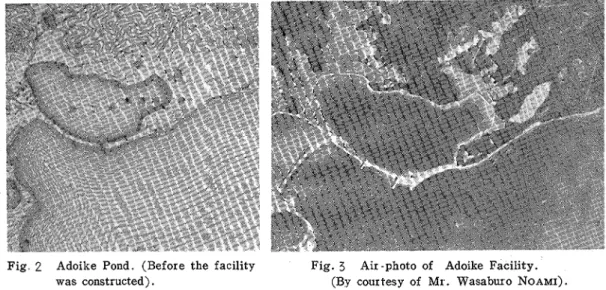
Wasaburo NOAMI, a pioneer of the shallow-marine cultivation of "Hamachis" (The young of Serzola quinqueradzata) in Japan in 1927.As shown in Fig. 1, there is a stone bank with two water inlets. This bank was constructed on the sand spit that runs from the northeastern sea cliff to t h e south along Hiketa Bay and i t forms this lagoon (Adoike Pond) as shown i n Fig. 2, and Fig. 3.
F i g 2 Adoike Pond (Before the facility Fig. 3 A ~ I -photo of Adoike Facility. was constructed). (By courtesy of M r . W a s a b u ~ o NOAMI). Fig. 2 is the map(2) showing Adoike Pond before the facility was constructed. From this map, we can see the sand spit with one tidal inlet. Fig. 3 i s the ai:.photo of Adoike Facility showing the sand spit along the bank. In 1964, to protect the bank from typhoons, the stone bank was covered with a concrete layer of 20 cm on the side facing the facility and 30cm on the side facing the sez.
The water inlet on the south side of the bank consists of hume pipes as shown in Fig. 4-A, and the water inlet on the north side of the bank consists of five water gates as shown in Fig. 4-B. A t the north gates, iron screens are used to prevent the fishes from escaping; and at the south water inlet, a fish-net i s used for the same purpose.
Tech. Bull. Fac. Agr .. Kagawa Univ.
V 104 m3
A 104 m2
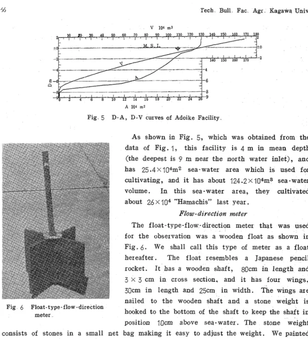
Fig 5 D. A , D - V curves of Adoike Facility
As shown in Fig. 5, which was obtained from the data of Fig. 1, this facility is 4 m in mean depth (the deepest is 9 m near the north water inlet), and has 25.4X 10⁴m2 sea-water area which is used for cultivating, and i t has about 124.2 x 10⁴m3 sea-water volume. In this sea-water area, they cultivated about 26 x 104 "Hamachis" last year.
Flow- dzrectzon meter
The float-type-flow-direction meter that was used for t h e observation was a wooden float as shown in Fig. 6. We shall call this type of meter as a float hereafter
.
The float resembles a Japanese pencil rocket. I t has a wooden shaft, 80cm in length and 3 x 3 cm i n cross section, and i t has four wings, 30cm in length and 25cm in width. The wings are nailed to the wooden shaft and a stone weight i s Fig 6 Float-type-flow -directionmeter hooked to the bottom of the shaft to keep the shaft i n position IOcm above sea-water. The stone weight consists of stones in a small net bag making it easy to adjust the weight. We painted each float a different color so that we could distinguish their position.
Observation
We used the Triangulation method to check the positions of the floats a s they moved along with the current. We used two Tokyo Kogaku A-type transit-theodolites. We set one a t point A on the stone bank near the south water inlet and the other a t point B near the north water inlet as shown in Fig. 1
.
We used a small fishing boat t o place the floats in the sea-water
.
As soon as t h e floats were placed in the sea-water, their positions were immediately checked by t h e two transit-theodolites. Their positions were checked every few minutes and they were later plotted on a map.With the above procedure, we conducted four observations a s listed on Table 1; 1) the period from 20:45 to 23:40 on August 13, 1965, during the flood tide of the spring tide,
Vol. 18, No 1 (??66) 37 Table 1 Observation date and the period
No Date Observation period Tide
-
--
1 August 13, 1965 from 20:45 to 23:40 Flood (Spr ing tide)
2 14, Ebb N
3 September 12, 8:36 12:55 Flood-ebb u
4 12, 14:26 18:05 Ebb //
2) the period from 3: 22 to 7:55 on August 14, 1965, during the ebb tide of the spring tide, 3) the period from 8:36 to 12:55 on September 12, 1965, during the flood-ebb tide of the spring tide, and 4) the period from 14:26 to 18: 05 on September 12, 1965, during the ebb tide of the spring tide.(')
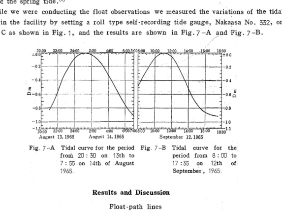
While we were conducting the float observations we measured the variations of the tidal level in the facility by setting a roll type self -recording tide gauge, Nakaasa No. 332? on point C as shown in Fig. 1, and the results are shown in Fig. 7 -A and Fig. 7 -B.
Fig 7 -A Tidal curve for the period Fig 7 -B Tidal curve for the from 20 : 30 on 13th to period from 8 : 00 to 7 : 55 on 14th of August 17:35 on 12th of
1965 September
,
1965Results and Discussian Float -path lines
From the four observations, we obtained four float-path line maps as shown in Fig.8- A, Fig.8-B, F i g . 9 - A , and Fig.9-B.
The float path line referred to h e ~ e is the line connecting the position of the floats measured by the transit-theodolites. Taking Fig. 8 -A as an example, we obtained the position of the float by simultaneously measuring the position as soon as t h e float was placed in the sea.water at 21:58 with the two transit-theodolites that were set a t points A and B and this was plotted as S1-1 on Fig. 8 -A. The next position taken a t 22:35 was plotted as S1-2 on the same figure and the following positions as S1-3, Sj-4, S1-5, and S1-6. We obtained line S1 by connecting the six points and this line is what we refer to as a path line: technically, this is referred to as the path of the float from 21 :58 to 23:40. Fig. 8 -A is the map obtained from the observation during the flood tide from 20:45
38 Tech. Bull.. Fac. Agr.. Kagawa Univ. to 23:40 on August 13, 1965, of the spring tide. Fig. 8 -B was obtained from the observation during the ebb tide from 3:22 to 7:E5 on August 14, 1965, of the spring tide. Fig. 9 -A was obtained from the observation during the flood-ebb tide from 8:36 to 12:55
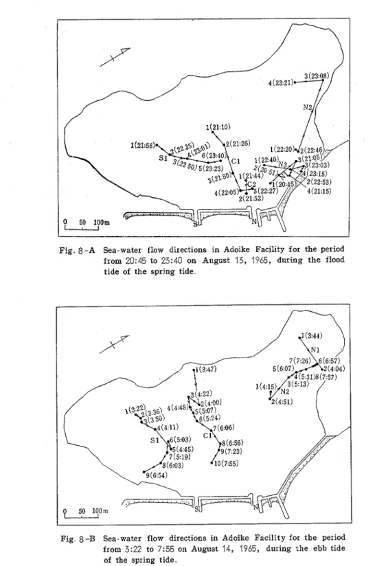
Fig. 8 - A Sea-water flow directions in Adoike Facility for the period from 20:45 to 23:40 on August 13, 1965, during the flood tide of the spring tide
Fig 8 -B Sea-water flow directions in Adoike Facility for the period from 3:22 to 7:55 on August 14, 1965, during the ebb tide of the spring tide.
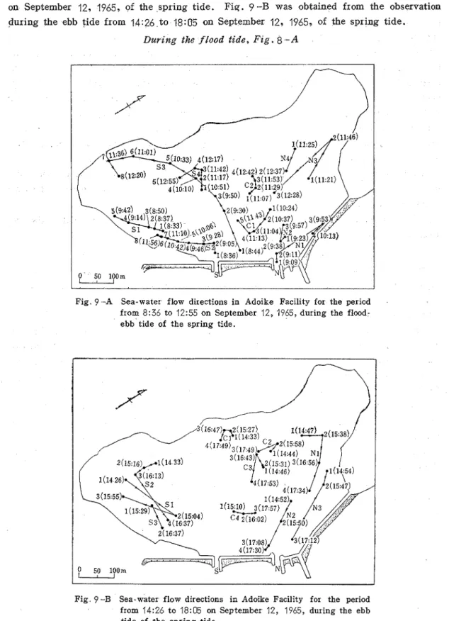
Vol. 18, No. 1 (1 966) 39 on September 12, 1965, of the spring tide. Fig. 9 -B was obtained from the observation during the ebb tide from 14:26 to 18:05 on September 12, 1965, of the spring tide.
During the flood tide,
Fig.
8 - AFig 9 -A Sea-water flow directions in Adoike Facility for the period from 8:36 to 1 2 5 5 on S e p t e m b e ~ 12, 1965, during the flood- ebb tide of the spring tide.
Fig 9 -B Sea-water flow directions i n Adoike Facility for the period from 1 4 2 6 to 18:05 on September 12, 1965, during the ebb tide of the spring tide
40 Tech Bull Fac Agr Kagawa Univ
Duping the flood tide, from 20:45 to 23:40 on August 13, 1965, six floats were used for the observation, and the result is shown as six path lines, path line N1, path line N2, path line N3, path line C1, path line C2, and path line S1 on Fig. 8 -A.
In the northeastern part of Fig. 8 -A, there are three path lines, path line N1, path line N2, and path line N3. These path lines show that the sea-water goes from the north water inlet to the northwest along the bank of the northeastern side of the facility. Looking at path line N1 from point N1-3 to point N1-4, and path line N3 from point N3-3 to point N3-4, the sea-water goes from the north to the south along the bank.
In the central part of the figure (the area between the south water inlet and t h e north water inlet), there are two path lines, C1, and C2. From these two path lines, the sea- water goes from the central part of the facility to the north water inlet.
In the south part of the figure, there i s path line S1. From this path line, the sea-water goes from the south to the northeast, and i t seems to be in a circular movement with a large radius
.
Looking a t path line S1, there also seems to be a large circular movement of the sea- water in the south-central part of the facility.
During the flood-ebb tide, F i g . 9 -A
During the flood-ebb tide, from 8:36 to 12:55 of Sepetember 12, 1965, 10 floats were used for the observation. The result i s shown as 10 path lines, N1, N2, N3, N4, C1, C2, S l , S2, S3, a n d S 4 , on Fig. 9-A.
In the north part of Fig. 9 -A, there are four path lines, N1, N2, N3, and N4. Looking at path line N1 from point N1.-1 to point N1-3, and a t path line N3 from point N3-1 to point N3-2, the sea-water goes from the north water inlet to the north. Looking a t path line N1 from point N1-3 to point N1-4, the sea-water goes from the north to t h e south towards the north water idtet along the northeastern bank. Frcm path line N3 from point N3-2 to point' N3-3 and path line N4 from point N4-1 to point N4-2, the sea-water goes from the north to the southeast towards the north water inlet. Therefore, from the above three path lines aad path line N2, the sea-water is in a circular movement in the north part of the facility.
In the central part of Fig. 9 -A, there are two path lines, C1 and C2. Both path lines show that the sea-water is i n a circular movement.
In the south part of Fig. 9 -A, there are four path lines, S1, S2, S3, and S4. From path lines, S1, and S2, the ses-water goes from the area near the south water inlet to the southwest along the southeastern bank. From path lines S3, and S4, the sea-water goes from the south water inlet to the southwest. Therefore, from these four path lines, the sea-water flows in two circles; one in a clock-wise movement along path lines S1 and S2. and the other i n a counter-clock-wise movement along path lines S3 and S4.
Durzng the f i r s t ebb tzde, Fzg. 8 -B
During the first ebb tide, from 3:22 to 7:55 on August 14, 1965, four floats were used for the observation. The result is shown as four path lines, N1, N2, C1, and S1, in Fig. 8-43.
Vol 18, No 1 (1966) 41
I n the north part of Fig. 8 -B, there are two path lines, N1 and N2. Path line N2 shows that the sea-water goes from the south to the north, but path line N1 shows that the sea-water goes from the west to the east.
In the central part of Fig.8 -B, there is path line C1. From this path line, the sea- water qoes from the west to the east; and it is in a circular movement.
In the south part of Fig .8 -B, there is path line S1. This path line shows that the sea-water goes from the west to the south and it is in a circular movement.
Durzng the second ebb tide, Fzg.9-B
During the second ebb tide, from 14:26 to 18:05, on September 12, 1965, 10 floats were used for the observation. The result is shown as 10 path lines, N1, N2, N3, C1, C2, C3, C4, S1, S2, and S3, i n Fig. 9-B.
In the northeastern part of Fig. 9-B, there are three path lines, N1, N2, and N3. These path lines are parallel to each other; and they show that the sea-water goes from the north to the southeast towards the north water inlet.
In the central part of Fig .9 -B, there are four path lines, C1, C2, C3, and C4. Path lines C1, C2, and C3 move in a counter-clock-wise circle, and they show that the sea- water in each path line is in a separate circular movement. Path line C4 shows that the sea-water flows parallel to the stone bank and is a part of a big circular movement.
I n the south part of Fig .9 -B, there are three path lines, S1, S2, and S3. Path line S1 f ~ o m point S1-1 to point S1-2, path line S2 from point S2-3 to point S2-4, and path line S3 show that the sea-water goes from the west to the east towards the south water inlet. But path line S1 from point S1-2 to point S1-3 shows that the sea-water flows from the east to the southwest, which indicates that the sea-water in this area also moves in a clock- wise circular movement.
From Fig .8 -A and Fig .9 -A, we estimated the flow directions of the sea-water during the flood tide and flood-ebb tide, and we drew up Fig.10-A.
During the flood tide, the sea-water flows in through the two water inlets, and it flows from the north water inlet to the north i n the north part of the facility; and along the northeastern bank, i t flows from the north to the south towards the north water inlet, and they all move in several circular movements.
In the central part of Fig.10-A, the sea-water flows in a circle as shown in Fig.10-A. In the south part of the facility, the sea-water flow forms two large circles; one is in the southeast and the other i s i n the southwest of Fig.10-A.
From Fig .8 -B and Fig. 9 -B, we estimated the flow directions of the sea-water during the ebb tide, and we drew up Fig. 10-B. During the ebb tide, the sea-water flows towards the two water inlets as shown in Fig.10-B, and the sea-water flows in a circle on this figure.
Sea- water velocity
From the data on the path lines that were shown i n Fig.8-A, Fig.8-B, Fig.9-A ,and Fig.9 -B, we estimated the mean velocity of the sea-water by using Eq. (I),
d l
v
= --." . . ..
42 Tech. Bull Fac Agr. Kagawa Univ. where d l is the distance (m) between a point and the adjoining point on the path lines, d t i s the time (min) that it took the float to move to the adjoining point on the path lines, and V (m/min) is the mean velocity of the sea-water between two points on the path line. V i s the mean velocity of the float i n dl, but we used it as the mean velocity of the sea- waterc3).
The procedure to obtain V is a s follows:
From the path line N1 on Fig.8-A, we get, the time 20:45 a t point N1-I, and 20:51 a t point N1-2; thus,
dt=20:51-20:45=6minutes...
. .-. ... .".
...
(A)and the distance between point N1-1 and point N1-2 on the same figure i s obtained a s 36m, thus,
d l = 3 6 m
... ...
. . . . . . . . .
a.
".
(En.
Substitutinq the values (A) and (B) for E q . ( l ) , we get the value of V,To measure d l or the distance between a point and the adjoining point on t h e figure, we used a dividers and a triangular -1 /400 scale.
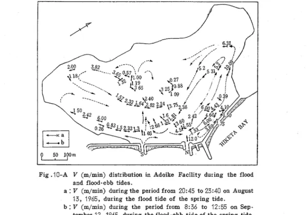
Using Eq. (I), we calculated V for all of the path lines on Fig .8 -A, Fig.8 -B, Fig.9 -A, and Fig.9 -B, and we drew up Fig.10-A and Fig.10-B. Fig.10-A shows the directions and distribution of V in the facility during the flood tide, from 20:45 to 23:40 on August 13, and during the flood-ebb tide from 8:36 to 12:55 on September 12, 1965.
Fig .lo-A V (m/min) distribution in Adoike Facility during the flood and flood-ebb tides.
a : V (m/min) during the period from 20: 45 to 23:40 on August 13, 1965, during the flood tide of the spring tide.
b : V (m/min) during the period from 8:36 to 12:55 on Sep- tember 12, 1965, during the flood-ebb tide of the spring tide.
Vol. 18, No. 1 (1966)
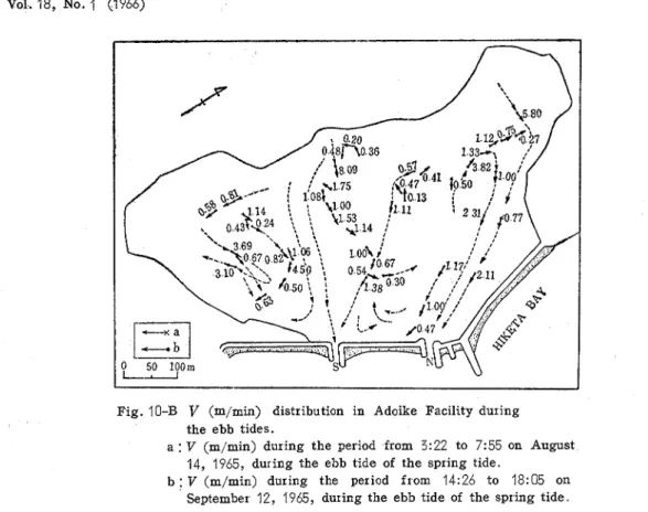
Fig. 10-B V (m/min) distribution in Adoike Facility during the ebb tides.
a : V (m/min) during the period from 3:22 to 7:55 on August 14, 1965, during the ebb tide of the spring tide
b : V (m/min) during the period from 14:26 to 18:05 on September 12, 1965, during the ebb tide of the spring tide
Fig. 10-B shows the directions and distribution of V in the facility during the ebb tide from 3:22 to 7:55 on August 14, and from 14:26 to 18:05 on September 12, 1965.
During the flood tide and flood-ebb tide (Fig.10-A), the magnitude of V varies from 12.0 m/min to 0.26 m/min. The highest 12.0 m/min is between point N1-1 a t 9:09 and point N1-2 a t 9:q-l near the mouth of the north water inlet on September 12. The lowest 0.26m/min i s between point S2-7 at 11 : 10 and point S2-8 a t 11 :56 near the south side of the facility on September 12.
During the ebb tides, the magnitude of V v a ~ i e s from 8.09 m/min to 0.13 m/min. The highest 8.09 m/min is between point GI-
1 a t 3:47 and point C1-2 at 4:00 near the lo west side of the facility on August 14. The lowest 0.13 m/min is between point N2-7 at 7:26 and point N2-8 a t 7:57 in
3
the north part of the facility on August > 14.Varzation of V
To find out the variation of V due to the
time and place, we drew up Fig. 11-A Fig. 11-A Variation of V (m/min), ~h (m/h), and D (m) for the period 20:45 to 23:40 from the data on Fig. 8 -A; Fig. 11-B on August 13, 1965, during the flood from the data on Fig. 8 -B; Fig. 12-A tide of the spring tide.
Tech Bull Fac Agr Kagawa Univ.
August 14,1965
t
Fig I I-B Variation of V (m/min), V h (m/h)
,
and D (m) for the period from 3:22 to 7:55 on August 14, 1965, during the ebb tide of the spring tide.f r o m t h e data o n Fig .9 -A; and Fig. 12-B f r o m t h e data o n Fig .9 -B.
Fig .I 1-A shows t h e variation o f V , V h and D during t h e flood t i d e , f r o m 20:45 t o 23:40 o n A u g u s t 13, 1965. X - a x i s i s t h e observation t i m e . Y - a x i s at t h e l e f t side of t h e figure i s V ( m / m i n ) , and y - a x e s a t t h e right side o f t h e same f i g u r e are V h ( m / h ) and D ( m ) . D i s t h e tidal level measured f r o m t h e sea-level at t h e h i g h t i d e t o t h e bottom o f t h e facility as shown i n Fig.7 -A and Fig.7-B V h i s t h e vertical velocity o f t h e sea level defined a s , d D Vlz
-
-. .
" . . .
. .
d t.
. ( 2 ) where d D i s t h e d i f f e r e n c e i n t h e D In d t , dt i s t h e d i f f e r e n c e i n t i m e . T h e procedure t o obtain V h i s a s follows:From t h e data o n Fig.7-A, w e g e t ,
-0.83 m as D at 21 :00 o n August 13, 1965 ( = D l ) -0.56 m a s
D
at 22:00 o n A u g u s t 13, 1965 ( = D 2 ) , t h u s ,dD=De-D1=-0.56m-(-0.83m)=O.27m,
and w e g e t , d t =22:00-21:00=1 hour, therefore, V h i s d D V h = - = 0 . 2 7 = 0 . 2 7 m / h . d t 1W h e n sea level goes u p , V h has a plus sign, and when t h e sea level goes down, V h has a minus sign.
In Fig.11-A, V h varies f r o m 0.27m/h t p 0.19 m / h while D varies f r o m -0.83m at 21:00 to -0.15m at 23:40.
I n Fig.11-A, t h e values o f V v a r y f r o m 10.09 m / m i n o n curve N2 (taken f r o m point N2-2 at 22:A6 t o point N2-3 at 23:08 o n Fig.8 -A) t o 0.39 m / m i n o n curve N2 (taken f r o m point N2-1 at 22:20 t o point N2-2 at 22:46 o n Fig.8-A). Since path lines N 1 , N2, and N 3 r u n through t h e north part o f Fig.8-A, and path lines C1 and C2 run through t h e central part o f t h e s s m e f i g u r e , and path line S1 runs through t h e south part o f t h e same
Vol 18, N o U 1 (1966) 45 figure, Fig.11-A shows that the sea-water in the north part of the facility flows faster than the sea-water in the other parts of the facility.
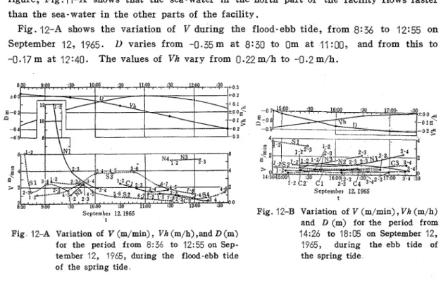
Fig. 12-A shows the variation of V during the flood-ebb tide, from 8: 36 to 12:55 on September 12, 1965.
D varies from -0.35 m a t 8:30 to Om a t 11 :00, and from this to
-0.17m a t 1?:40. The values of Vh vary from 0.22m/h to -0.2m/h.September 12,1965
September 12, I965
t
Fig. 12-B Var iation of V (m/min)
,
V h (m/h)t and D (m) for the period from
Fig 12-A Variation of V (m/min)
,
V h (m/h) ,and D (m) 14:26 to 18:05 on September 12, for the period from 8:36 to 12:55 on Sep- 1965, during the ebb tide of tember 12, 1965, during the flood.ebb tide the spring tideof the spring tide
On Fig. 12-A, the values of V vary from 12.0 m/min on curve N1 (taken from point N1-1 at 9:09 to point N1-2 a t 9:11 on Fig.9 -A) to 0.26 m/min on curve S2 (taken from point S2-7 a t 11 :I0 to point S2-8 a t 11 :56 on Fig .9 -A). Curves N1, N2, and N3 and point N4 have larger values of V than the other curves. Since path lines N1, N2, N3, and N4 are in the north part of Fig.9 -A, the sea-water in this part flows from the north water inlet to the north with a higher velocity th2.n in the other parts of t h e figure. Curve S3 has a larger value of V than curves C1 and C2. Since path line S 3 is in the south part of Fig. 9-A, and path lines C?, and C2 are in the central part of Fig.9 -A, the velocity of the sea- water in the south part of Fig .9 -A i s higher than the velocity i n the central part of Fig.9 -A. Therefore, during flood-ebb tide, and flood tide, the sea- water in the north part of the facility has the highest velocity in the facility.
Fig.11-B shows the variation of V, Vh, and D during the first ebb tide, from 3:22 to 7:55 on August 14, 1965. The values of Vh vary from -0.19m/h to -0.17m/h while D varies from -0.33 m a t 4:00 to -0.91 m a t 7:00. The values of V vary from 8.09 m/min on curve C1 (taken from point C1-I a t 3:47 to point C1-2 at 4:00 on Fig.8 -B) to O.lgm/rnin on curve N2 (taken from point N2-7 at 7:26 to point N2-8 a t 7:57 on Fig.8 -B)
.
During the period from 5:40 to 8: 10 the values of -V on curve C1 are larger than on curves N2 and S l.
But during the period from 4:30 to 5:00, the values of V on curve N2 are the largest of all curves that are shown in the figure.Fig. 12-B shows the variation of V , Vh, and D during the second ebb tide, from 14:26 to 18: 05 on September 12, 1965. The values of Vh vary from -0.18 m/h to -0.01 m/h while the values of D vary from -0.71m at 14:50 to -0.91 m at 17:30. The values of V vary
46 Tech Bull. Fac. Agr Kagawa Univ from 3.69 m/min on curve S1 (taken from point S1-1 at 14:26 to point S1-2 a t 15:04 on Fig. 9 -B) to 0.76 m/min on curve C3 (taken from point C3-1 a t 14:46 to point C3-2 a t 15: 31 on Fig .9 -B)
.
The values of V on curves N1,
N2, and N3 are larger than the values on the other curves. Since path lines N1, N2, and N3 run through the north part of Fig. 9 -B, here again this shows that the sea-water in the north part of the facility has the highest velocity in the facility. Although the velocity during flood tide (Fig.I 1 -A, and
Fig.12-A) is much higher than the velocity during ebb tide, Figures 11-B and 12-B also show that the north part of the facility has the highest velocity i n the facility.Since the amount of the exchange of sea-water between the facility and the sea depends mainly on the velocity of the sea-water, the north part of the facility has the best exchange rate, especially, during the flood tide.
Summary
To find out the flow directions of the sea-water that flows into the facility and in the facility, float-observations were conducted at Adoike Facility, Kagawa Prefecture during one flood tide (from 20:45 to 23:40 on August 13, 1965), and during cne flcod-ebb tide (from 8:36 to 12:55 on September 12, I%), and during two ebb tides (frcm 3:22 to 7:55 on August 14, and from 14:26 to 18:05 on Septtmlxr 12, 1965). The prccedures and results are as follows:
1) To observe the flow direction of the sea-water, several wooden floats were used, and to measure the positions the Triangulation method was used with two transit-theodolites.
2) During the flood tide, the flow of the sea-water that flowed in through the two water inlets are shown in Fig.8 -.IS. and Fig.9 -A; and during the ebb tide, the flow of the sea- water that flowed towards the two water inlets are shown in Fig.8-B and Fig.9 -B. 3) The velocity of the sea-water that flowed into the facility and in the facility varies from 12.0 m/min near the north water inlet to 0.26 m/min at the south part of the facility during one flood tide and one flood-ebb tide. The velocity of the sea water that flowed out of the facility varied from 8.09m/min in the central part during cne ebb tide to 0.13 m/min also in the central part during the other ebb tide.
4)
The variation of the velocity of the sea.water during the tides are shown in Fig. 11 -A for the flood tide, Fig.12-A for the flood-ebb tide, Fig. 11-B for the first ebb tide, and Fig .l2-B for the second ebb tide.5)
During both flood and ebb tides, the sea-water in the north part of the facility has the highest velocity i n the facility, especially, during flood tide.6)
During both flood and ebb tides, there are two dead-water zones in the facility; one is in the north side along the edge of the facility and the other i s in south side along the edge of the facility.
Acknowledgements
The writers wish to thank Mr. Wasaburo NOAMI the former. director of Adoike Facility for his help for this investigation, and Professor Minoru SAITO of Kagawa University for his suggestion concerning this work, and Mr. Hachiro AOZU, Mr. Taizo SATO, and Ms.
Vol. 18, No. 1 (1966) 47 Katashi KODERA former students of Kagawa University for their help in the observations, and also Mrs. Chieko MATSUBARA a member of our laboratory for her assistance for this work.
References
(1) KAIJOHOANCHO SUIROBU : NazkaZ' Chosekih yo, (3) ROUSE H. : Engineering Hydraulics, 193, Third
K2 14-1 5 (1 965) printings (1961) John Wiley & Sons, Inc New
(2) KOKUDOCHIRIIN : Topographic-map, 1 /50000 York.
Hiketa (1 947)
$52 P : &&Z%%%KaaK&@7k/X@10&BB7 B&$EBB&B?Z3t%kG?LZ3.
%F%
(%)llLRAJll%GlBlm) % ~ E B % % o R S N % 8 I r
L,
c
o%%K aaK6??47k%@, Ir<
b@7k%Bo@@Q1965+ 8B
13, 148 ( L V B , T V B ) , It398
128 (_tV%I-.TVB, T V B )o
4 El (b~.P'?L&AB@), ucbk 0 Float &%r;iJHKk 9