Transient Behaviour of The Mean Waiting Time and Its Exact Forms in M/M/1 and M/D/1

Vo!. 19. No. 1. March, 1976

TRANSIENT BEHAVIOUR OF THE MEAN

WAITING TIME AND ITS EXACT

FORMS IN

M/M/1

AND

M/D/1

MASAO MORI Ibaraki University

(Received October 4, 1974) Abstract

The qualitative natures of the transient behaviours of the waiting times in a GI/G/l system are studied first, when the waiting time of the initial customer is

v.

For instance, it is shown that the mean waiting time is in-creasing in n only when v < l for some l.

Next this paper gives a way of calculating exact values of the mean wait-ing time of the n-th arrival in M/M/l and M/D/l and further proposes a simple scale of the rate of convergence to the equilibrium state.

1. Introduction and preliminaries.

Many authors have written papers on the subject of transient behaviours of queueing systems until now. Some of them have derived exact finite time solutions for simple queues (see Cohen [2]). Some of them have studied on the rate of convergence -- the exponential convergence -- to the equilibrium state (see Vere-Jones [17], Heathcote [10] and Miyazawa [12]). And some of them have checked the decreasing rate of the serial correlation coefficients of waiting times and have utilized the results to evaluate errors in estimat-ing the mean waitestimat-ing time by usestimat-ing sample averages on simulation experiments

(see Daley [3] and Blomqvist [1]). Certainly their works give important and worthy informations on the subject to the practical researchers and the theo-reticians.

From another standing point, Davis [5J introduced "the buiZd-up time" as a rough scale of the rate of convergence to the equilibrium state. And, for a M/G/1 system, Morimura I13J conjectured that the queueing process may be con-sidered to have almost reached at equilibrium state after the lapse of about two times of the build-up time Tb starting from the empty state, where Tb

=

fa

t'dEv(t) / Ev(oo) and v(t) is the virtual waiting time at t. This result also proposes a convienient and valuable measure to the practical researchers.

But it was reported by Hashida [9J that for the M/M/k system the build-up time

Ti

3 starting from the state where there are

i

customers in the system

Transient Behaviour in Jf! MI 1 and MI DI 1 15

initially, may take a negative value. For example T. is negative in the

1-case of the traffic intensity p

=

0.4. The reason why T. may take a nega-

1-tive value is because the mean system size does not necessarily increase mono-tonously and may be fluctuating. So we think that it is necessary to investi-gate the grobal properties of transient patterns of queueing processes.

In this paper we will first consider 3. GI/G/I queueing system with first in first served (FIFS) discipline. Let t _r;. be the interarrival interval be-tween the {n-l)-th and the n-th arriving customers; {t, n

=

1, 2, ... } is a

n

sequence of positive i.i.d. variables. And the service time of the n-th arriv-ing customer is denoted by s ; {s , n

=

C, 1, 2, ..• } is also a sequence of

n n

positive Li.d. variables. And we denote by w (v) the waiting time of the n

n-th arriving customer when the system starts from the initial condition that there remain total residual service loads of

v

at

t

=

0, i.e.

Wo

= v.

Now we would want to know the qualitative nature of the transient behaviour of the process

{w

(v), n

=

1, 2, ... }, and, in particular, we are interested in

n

the mean waiting time Ew (v)

n as functions of n for different initial values of

v.

For example, we can show Ew (v)

n is increasing in

n,

if

v

is smaller than some value

l.

In the section

3,

we give the explicit forms of

P{w

(v) = O} n

and M/D/I, and by using them we can calculate the exact values of cursively to study the transient behaviour more concretely.

in M/M/I Ew (v)

re-n And for these case, we will examine numerically some scales of the rate of convergence to the equilibrium state, when the process starts from

Wo

=

O. In those scales. '2

=

(o~

+

pot) / (1 - p)2 seems to be a favourable one, where 0a and ob are the coefficient of variation of the inter-arrival times and the service times respectively and p is the traffic intensity. Trans-forming the number n of the n-th arriving customer into n'

=

n/'2' the val-ues of y~, = [Ewn(O) / Ewoo] x 100 % for M/D/I behaves almost similarly to those values for M/M/I, where y~, is considered to represent a measure of measuring "the oloseness to the equilibrium state." And it is shown that y~,

~ 95 % for

n'

=

2 for both cases. Other time transformations such as stat-ed above have been dealt with by Gaver [8] and Newell [14] in the study of dif-fusion approximations of queueing processes.

Here we are summing up preliminary definitions and a lemma for later use. 1. (EsapY, P1'Osohan and Walkup [6].)

Random variables (Xl' X₂, ... , Xn) a~e said to be assooiated if

for

every pair of functions f and g which are monotone non-decreasing in each arguments~ provided that the covariance exists.

It is noticed that mutually independent random variables are of course associated.

2. Let

£

be the family of real valued random variables with finite mean on a probability space.

We define the following binary relation on X x '£ ,which are introduced by H. Stoyan and D. Stoyan [16] to investigate the order relationships between some queueing systems.

Definition. (Stoyan) For any Xl and X₂ E L , we denote Xl C X

2 if (1.2)

r:

_P{Xl >

x}dx

~

J:

P{X₂ >

x}dx

c c

for

all c.

Lemma. (a) If Xlc X

2 and X2c X3' then Xlc X3 (Trasitivity). (b) If X3 is independent of Xl and X2~ then Xlc~ _{X2 implies Xl}

+

X3

c:

X

2 + X3•

(c) If Xlc' X2~ then max(O, Xl)c max(O~ _X2).

(d) If Xlc= X2~ then EXl ~ EX₂· Particularly in the case of Xi > 0 and E~ < 00

for

i

=

1, 2~ we have

EX;

~

EX;

(e) Let P{X

1

=

a}

=

1. Then we have X1c: X2

for

any X2 such that EX2

=

a. And many other interesting properties are shown in [16]. Here we add one new property which gives us useful information to compare queueing systems.

(f) Let {X.} be a sequence of i.i.d. random variables. _-z, Then

(1.3)

[1] .

i

Y.=

L

X . / i -z, j=l J

This property is proved by the similar way as deriving equation (3) in

In this paper we often say that Xl is smaller than X

2 in the Stoyan's sense if X

1C-X2. Notice that this definition is a natural extention of the ordinary stochastic order, which we denote

x

l S

!·X₂ if P{X

l > x}

~

P{X2 > x}.

2. The transient patterns of the

{wn(v)}

process.

2.1 The

{w

(v)}

process.

Transient Behaviour in Mj Mj 1 and Mj Dj 1 17 section. Let

w

be a typical random variable which obeys to the equilibrium waiting time distribution W(x) if it exists. Let G(x) be the d.f. of u

n n

=

8 -

t

n+1, and let V

=

L

u . . Hence we have

n n i=O ~

(2.1)

w

_n+_{1 (v)} = max(O, wn(v)

+ un)

from which we can easily derive

For any fixed

n,

let us put u 1 = u 1 .

~ n- -~

1, 2, ... , n-1. Then we can rewrite (2.2) as (2.3) _Wn(v)

=

max(O, _{Vo ' V1 '}

*

_*

...

"

V* _n-l

+

v)

=

max(O,

*

*

V* ) V 0 ' V1 '

...

"

n-l foY' n ~ 0,

i

*

I;'

*

and V. = L u. 1.- j=O J

+

max(O, v + V* ma:r(e,

* *

n-l

-

VO ,V1 '

...

"

= wn(O) + [v + mix(O, V_O' V 1' ... , Vn_1 )]+ for

i

= 0,

with probability one, where [a]+ = max(O, a). And it is noteworthy that the last term is stochastica11y equal to

[v -

W

]+, i.e.

n

(2.4) M v ( ) == [ v

+

m1.-n 0, VO' ... , V _, . ( )]+ 'V [ V - Wn ' A]+

n-j

where

{w}

_n is the waiting time process of the dual queueing system generated by interchanging the service time distribution and the interarriva1 time dis-tribution of the original system each other, in which the process is assumed to start from the state

Wo

=

O. Of course Wn(O) and M(v) are highly cor-related, but as for the expectation we can write

(2.5) Ew (v) = Ew (0)

+

E[v - W ] A

+

n n n

Hereafter we assume that the original system satisfies the equilibrium condi tion -co < E (u

O) < O. So the dual queueing system turns out to be a

di-vergent queueing system.

2.2 On the transient patterns.

At first we will sum up the results obtained by B10mqvist [1] on the tran-sient pattern of {W

n (O)} process when 1) = O. Let us denote Wn (0) by wn

Proposition 2.1 (Blomqvist)

st. st. st.

(i) {U)n} 1:S stochasticaUy increasing in n, i. e. nO ~ 1J

1 ~ U)2 ~ Further there exists at least one x such that the strict inequality

P{U)n ~ x} < P{U)n+1 ~ x} holds.

(ii) {EU)} is strictly increasing and concave in n. n

(iii) {var(U))} is also strictly increasing in n. _n Next we will state on the transient patterns of the First we get the following rather trivial results.

{U) (v)} process.

n

Proposi tion 2. 2

(i) U)n(v) is stochastically increasing in v for all n.

(ii) EU)n(v) is strictly increasing in v for all n.

(iii) var(U) (v)) is also increasing in v for all n. _n

Proof. (i) and (ii) are trivial from (2.3), and for more general queueing systems such as G/G/k with Markovian inputs analogous results may be derived by using stochastic monotonicity of the Markov chain (see Daley [4]), Now we will prove (iii). From (2.3) we get

(2.6) var(U) (v))

=

var(U) ) + Var(M(v)) + 2cov(u) , M(v)).

n n . n

A +

From (2.4) we have var(M(v)) = var([v - U) ] ) _n and

(2.7)

~v

var([v -

W

]+) =

+

{Jv(V - x)2dF (x) - (Jv(V - x)dF (X))2}

a n aV 0 n O n

= 2(1

where F _n (x) is the d.f. of it is enough to show that

- Fn(V))oJ:(V - x)dFn(x)

~

0

hence var (M (v)) is increasing in v.

(2.8) COv(U)n' M(v+!:::.)) - COV(U)n' M(v)) = COV(U)n' M(v+!:::.) - M(v)) ~ 0

Thus

for any !:::. > O. Now from the definitions of U) _n and M(v) , they can be re-garded as functions of the associated random variables

Clearly, U) _n is monotone non-decreasing in each U ••

'l-(u O' u1, u2' ••• , And M(v+!:::.) - M(v) u 1)'

n-is also monotone non-decreasing in each

is monotone non-decreasing in each u.

'l-u., since m

=

min(O, V_O' ... , V 1

'l- + n- +

and M(v+!:::.) - M(v)

=

(m+v+!:::.) - (m+v) is so in m. Thus, (2.8) is assured from the definition of association.

Proposition 2.3

(i) The difference all v.

(ii)

Proof·

Transient Belmviour in M/ M/I and M/ D/I And the difference

all v.

(Ew

(v)

n

Ew)

n is strictly decreasing in n for

(i) is :immediately deduced from (2.3). The "strict" decreasingness

19

in (ii) is derived from the later assertion in Proposition 2.1 - (i), which is also true for W • "

n

The above propositions are shown by using the ordinary stochastic order, but we need the Stoyan's order in the following further discussion.

Proposition 2.4

If v;,

Ew,

then there exists at lC2st a stochastically increasing se-quence of random variables {w ' } _n such th2t (A)

Ew

I = v and w (v) w I for

o

n n

all n and that (E) it has the same lim1:ting distribution W(x) as {w (v)}.

n And [w ' is strictly increasing in n in this case. _n

If v >

Ew,

then there exists at lC2st a stochastically decreasing {w ' } _n such that it has the same properties (A) 2nd (E) as above, but

ly decreasing in n in this case.

Ew

I is strict-n

+

Proof· Let us define {w~} recursively by w~+l (w~

+ Un)'

where

Wo

is any non-negative random variables satisfying EwO v and {un} is the same sequence as in generating

{w

(v)}. Then we can recursively show that

+ + n

w~+l

=

(w~ + un) (wn(v) + un)

=

_wn+1(V) holds for each n from the pro-perties (a), (b), (c) and (e). Thus (A) is ascertained for any

Wo

such that

EwO

,=

v.

And (E) is also true from the clefini tions of {w~}.

Now the remaining subject is how to determine

Wo

so as to make

{w

l }

EwO

=

v. Let

Wo

be the random

Ew,

or such that

w'

~

(w

+ c')

stochastically increasing or not subject to variable such that

Wo

~ (w - c)+ if

v;

i f v >

Ew,

where w is a typical random variables with the d.f. W(x) and the constants c

case. Of course, and it

Ew '

_o

=

v may hold for each and c' satisfying EwO

=

v, for E(w - c)+ and

c' are the values such that is possible to choose such c

E(w

+

c') are continuous in c and c' respectively. Then, it is easily seen after a little calculation that

_w'

decreases

stochas-n

tically in n if v > Ew and increases if v < Ew. And choosing

Wo

as above, the strict increasingness or decreasingness of

_{Ew '}

_n are easily shown.

However, we do not know yet what conditions should be putted upon w' ₀ in order to make a sequence {w I}

n stochasti cally increasing in n or, further, increasing in the Stoyan's sense. Let

vi

(x)

n be the d. f. w' n' and we have (2.9)

which is the Wiener-Hopf equation first derived by D.V. Lindley. First, by using (2.9) iteratively it is soon noticed that,

creasing in n, i.e.

{W

(x)} is decreasing in n n

WO(x) ~ W₁(x) for any x. Analogously from (b)

{w'}

is stochastically

in-n

for each x, if and only if

and (c)

{w'}

is increasing

n

in the Stoyan's sense if and only if

wOC= w1.

Thus the problem is reduced to finding the condition WO(x) ~

W

1(x) or WOc W

1

holds. Of course,

simi-lar results are also deduced concerning the decreasingness of

{w'}.

n

Here Some sufficient conditions are easily found: if WO(x) ~ G(x) for all x, we have Wo(x) ~ W₁(x) for all x. And if WO(xJ is represented as

WO(xJ = aG(x)

+

(1-a)W(x) for some a (0 ;, a ;, 1), we have also WO(x)~ W 1 (x)

In these cases, wOe w

1 also holds. However, the condition WO(x) ~ W(X) for all If: does not necessarily imply that WO(xJ ~ W

1 (x) for each x. For

example, for any fixed e > 0, let WO(xJ

=

W(x) for x > e and WO(x)= W(e)

for 0 ~ x < e. Then, after a little calculation, it is seen that WO(x);, W 1(x)

for each x such that x ~ e, and in this case woc w

1 does not hold. But, if we define WO(x)

=

W(x) (x < c);

=

1 (x ~ c), wOC=

w

₁ holds but WO(x)~ W

1(x)

does not for any

c.

And from Proposition 2.6 stated later, if WO(x)

=

0 (x < v); = 1 (x ~ v) and v is smaller than some value Z, wOe w₁ holds. So it may be expected that the transient behaviour of the waiting time in the global sense greatly depends upon whether WO(x) ~ W(X) for large value of x or not.

2.3 Transient patterns of

{Ewn(v)}.

Hereafter, we will concentrate only upon the transient patterns of the expectation value of the

{w

(v)} process and investigate them in rather detail.

n

L.et Z be a solution of the equation

r

(1 - G (y J Jdy = x. I t is known

-x

that

Z

is the unique solution of this equation and

Z

~ Ew ([11]). And from the following propositions it will be seen that

Z

is also a critical point for initial values of the waiting time process.

Proposition

2.5 (2.10)

Proof·

(2.11) By using (2.9), we have

if v

~ Z (~) Ew 1(v)

=

fOO

(1 - G(x))dx

= (

foo

+

f-Z

)(1 - G(x))dx -v -Z -v

Transient Behaviour in Mj Mj 1 and Mj Dj 1

=

Z

+

rz

(1 -

G(x))dx.

-v

Since (1 - G (x)) < 1 in the above, we obtain (2.10). Proposition 2.6

If v ~ Z, then

EW

(v) is increasing in n

n

increasing in the Stoyan's sense.

and further {W (v)}

n is

Proof. From Proposition 2.5 we have Ew₁(v) ~ v. Regard Ew₁(v) as a random variable taking a constant value, and

vc:::

Ew

1(v) C w1(v) holds from the property (e). IIence from (h) and (e) the relation w

1 (v) = (v

+

u

o

)+ '" (v

+ u

1)+ c: (w1(v)

+ u

1)+ = wiv) is obtaind. Through the same arguments, we have wn (v) c:: w

n

+

1 (v) for all n, which completes the proof.

21

Now the fOllowing open questions occur to us: whether does Ew _n (v) oscil-late in many times or not for v > Z ? ; whether does Ew (v) a'Pproach to Ew

n

from above or not for large v? We cannot answer here the above matters at all.

However, from examples stated in the last of the section 2.2 and so on, i t is conjectured that

Ew

(v) !:lay once decrease beyond Ew and gradually

n

increase to

Ew

from below for any large

v.

Further, it is conjectured that Ew' may approach to Ew from below for large n, if there exists x < 00

n 0

such that

P{w

_O

~ ~} >

P{w

~

x}

for any

x

>

xO.

In the next section, we shall show a way of calculating exact values of

Ew

(v) for M/M/l and M/D/l and study the transient behaviours of them more

n

concretely.

3. Transient solutions for M/M/l and M/D/l.

3.1 The fundamental relations for M/G/l.

In this section we are going to obtain the exact forms of the mean wait-ing time of the n-th arrivwait-ing customer for the systems M/M/l and M/D/l and to examine their transient behaviour in detail. For later use we prepare at first a few fundamental relations for M/G/l without proof. These relations are anal-ogously derived as in [2] (pp. 249-255).

Let

A be the arrival rate of customers and

B(x) be the d.f. of the ser-vice times. As the recurrence relation for the mean waiting times of the suc-cessive customers we have

(3.1) Ew (v)

=

Ew l(v) -

I

(1 - p) +

I

P{w (v)

=

o}

n n- A A n

and Ew O(v) = v. So we can calculate EW

n (v), i f the exact values of P{wn (v)= O}

(n

=

13 23 ••. ) are in hand. Now we consider the way of obtaining the value of a (v)

=

P{w (v)

=

a}.

n n

Let r(v) be the number of customers served in the busy period initiated by the O-th customer whose residual waiting time at the time 0 is

v,

i.e.

Wo

=

v.

by R(z)

And let Rv(z) be the generating function of r(v)

simply. If p < 1, then we have

and denote

(3.2) Rv(z) = z'e-AVU-R(Z)) • S[U - R(z))]

for

Izl

< 1, where S(8) is the Laplace transform of B(x). And R(z) sat-isfies the functional equation

(3.3) R(z) = Z'S[A{1 - R(z)J]

and we have

(3.4)

f

oo (Ax)k-l e-

A

% dBk*(x)

P{r(O)

=

k}

=

0 k!

where Bk*(x) is the k-fold convolution of B(x).

Since a (v)

=

P{w (v)

=

O} is considered as the renewal density at the

n n

time n of the delayed renewal process generated by random variables r(v)

and r(O), thus we have

00

(3.5) Q(z) -

L

n=l

for

Izl

< 1. The value of a (v) n pans ion of this generating function.

00

L

e -Av(l-R(z) ) • k=l

n is just the coefficient of z

3.2 The value of

P{w (v)

=

O}

for M/M/l.

n

in the

ex-Let ~ be the service rate. In this case the system size process ob-served at each arrival and departure time points is regarded as a one dimen-sional random walk with an reflecting barrier at the origin which are gener-ated by transition probabilities Pi

3i+l

=

P

=

A

~ ~

=

Tfp,

Pi ,i-l

=

1 - P = 1

!

p (i

=

1, 2, 33 " ' ) 3 P01

=

1 and POO

=

O. Thus we have n (3.6) P{r(O)

=

n}

= - -1 2n - 2 n - 1 n-1 p ) (1+p)2n-1

Transient Belwviour in M/ M/land M/ D/ 1 23

which is the probability of the first return to the origin at the time 2n

through the positive axis in the random walk. And let Rkn be the coefficient

of

zn

in the expansion of

{R(z)}k,

then we have

n-k

R _ k (2n-k) p

kn - 2n - k n (1

+

p) 2n-k

(3.7)

which is the probability of the k-th return to the origin at 2n (see Feller [7] p. 77.) Of course, above probabilities can be also obtained by expanding

{R(z)}.

Rewriting 0.5) as (3.8)

, R ( ) k , 0 0 k 00 ( , ) j .

el\V z {R(z)} = e-I\V

L

{R(z)} •

L

_I\_~- {R(z)}J

k=l j=O JI 00 -AV ~ Q(z)

=

e !.. k=l 00 k-1 j =

L

{R(z)}k

L

(A~~

e-AV, k=l j=O J. then we have (3.9) n

L

_Rk k-l

L -.,-

(v)j _e

-AV

k=l n j=O J. Proposition 3.1

For the system M/M/1,

if

P < 1 we have

n k k k k-1 ( , ) j ,

P{

_w

_{(v) = 0} } _{= L} ~ _{2 k} (2n _.) p _{2 k L} ~ _{- ' - , - e} I\V -I\V

n k=l n - n (1 + p) n- j=O J.

(3.10)

Especially in the case of v:: 0, after a little calculation we can re-write (3.10) as

n - 1 . n - 2 .

1

{L (

-E...)'1-(-~) _..2-..- ~ (--E- )'1-( -n-1

)l

(3.11) P{w = O}

n _{{l+p)n i=O l+p '1- l+p i~O l+p i '}

and we "an see P{w = O} - (1 - p) as n _ 00 •

n

The exact value of Ew (v) can be calculated recursively by using (3.10)

n

and (3.1).

3.3 The value of P{w

(v)

=

O}

for

MIDIl .

n

Let b be the service time. Since S(9) :: e -9b ,from (3.2) 'V (3.5) we have

(3.12) (3.13) R ( ) v z :: ze - (AV+p) (1-R{z)) , 00 R{z) = ze- p (l-R{z)) =

L

i e - kp k=l {kpyk-1 k!

and (3.14) 00 R v(Z){R(Z)}k-l 00 Q(z)

_L

_l

Z e k -(Av+kp)(l-R(z)) k=l k=l 00 k - (Av+kp) 00 (AV+ke)j _{R(z)}j =

I

z e

_I

.

,

k=l j=O J. By expanding (3.14), we get n-l a (v)

=

e-(AV+nP) {1 +

I

n k=l n-k e(n-k)p

l

j=l (AV+kei R j! j ,n-k },

and, replacing n-k by

k,

we have

n-l

k

a (v)

=

e-(Av+np) {1 +

I

ekp

I

n k=l j=l (3.15) [AV+ (n-k) _j! p]j R _{jk },} where Rjk (1 ~ j ~ k) is given by

v.-l

(3.16) j

(v.

p) 1- -v.P

IT

1- 1-V .! e

i=l

1-from (3.13). Putting

k.

=

v. -

1, we can rewrite (3.16) as 1- 1-(3.17) Rjk

=

e-k p • p k ' -J •

I

TT

j k 1+ ... +kj=k-j j=l k.>O 1-= k.-l (1+k.) 1-k ./

1-In order to simplify this, lve use the following mu1 tinomia1 Abe1 identity given in Riordan [5] (p. 26): (3.18) = (x • x • 1 2 • x. J

;-1 .

x • (x + n)n-l where x

=

xl + x 2 + .. , + Xj .

Now applying this identity to the last term in the right side of (3.17), we get

(3.19) _Rjk = e -kp • p k-j -;:;-....::;1:--:-7 • _{(k-j) /} j . k k -j -1 ,

and putting this into (3.15)

n-l k-l

a (v)

=

e-(Av+n p) {1

+

l {

(AV+ne) _ p} (Av+np) },

n k=l k (k-l) /

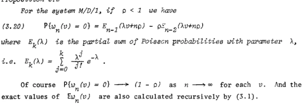
Transient Behaviour in Mj MjI and Mj DjJ 25 P1>opo8ition 3.2

For the 8Y8tem M/D/l, if p < 1 we have

(3.20) P{w (v)

=

O}

=

E 10.v+np) - pE' 2 (Av+np)

n n-

n-where Ek(A) i8 the partial sum of Poisscn probabilities with parameter

A,

Of course P{w (v) =

O}

~ (1 - p) as n ~oo for each v. And the

n

exact values of Ew (v) are also calculated recursive1y by (3.1).

n

3.4 Numerical examples for

{Ew

(v)} . n

According to the discussions until now, we can draw graphs of {Ew (v)} n

for different values of

v.

Figure 1 is the graph in the case of M/D/1 with p = 0.6, which shows typical transient pa.tterns of {Ew (v)} for every p.

n

And the graphs in the case of M/M/1 are also similar to this.

Fig. 1. 1.8,t Ew (v) n The graph of Ew (v) n for M/D/1 (p=O.6).

In this case,

Ew

_n (1.50) attains its minimum 0.99430 at n=11 and Ew (1.80) attains its minimum 0.9999930 at n=45. Here 0=Ew=0.750.

It is noteworthy that the value of P{w (v) = O} converges more rapidly

n to its limiting value

1-p

than

Ew

(v)

n does, which is naturally expected from the recursive relation (3.1) for the mean. This fact suggest to us that when we apply Markov model to a queueing system and estimate some quantities by multiplying the transition matrix with itself by a number of times recur-sively, percentiles of the distribution may be estimable more exactly than the moments values. On the other hand, "hen we must judge whether a practical queueing processes are considered to have reached at the equilibrium state or not, it may be more safe to judge from informations concerning the convergence rate of the mean waiting time than to use those of probabilities.

Now let us consider the unsolved question mentioned in ,the last of the section 2: for any value of v ~

Ew,

may

increase gradually to

Ew

afterwards?

Ew

(v) once decrease beyond

Ew

and n

In the case of M/G/l, from (3.1) this statement is rewritten as follows : for any value of v, may P{w (v)

=

O} ever

n

excess over its limiting value

1-p

and never cross down the value

1-p

after-wards?

However, we cannot make definite theoretically whether this statement is true or not even in the case of M/D/l and M/M/I. So we are going to examine this numerically. Certainly,

Ew

(v) behaves as in the manner stated in the

n

above statement, if v is smaller than 1.6 ~ 1.8 times of

Ew

for p

=

0.1

~

0.9(1) in the both systems. But, Ewn(v) seems to be monotone decreasing to

Ew,

if

v

is larger than these values. For example, in the system M/D/l with

n

=

4

p = 0.4, for v 1.5 and attains its minimum

Ew,

Ew

(v) goes accross n

0.9973 x

Ew

at n

=

6,

Ew

from above at and afterwards it in-creases to

Ew;

for v

=

1.8 x

Ew,

Ew

(v) attains its minimum 0.9999991 x

Ew

n

at n

=

21 and then increases; but, for v

=

2.0 x

Ew.

it is monotone decreas-ing to

Ew

and stays at

Ew

after n

=

30. To our regret we cannot judge whether this behaviour is owing to computational errors or not.

Anyway, in a practical sense we are allowed to consider that be monotone decreasing in n, if v is larger than above 2 x

Ew.

3.5 On some time transformations.

Ew

(v) may n

In the studies of diffusion approximations of queueing processes, a trans-form of the time scale and the queue length leads to a simple dimensionless

(1) We have computed the values

Ew

(v) only for p v

=

0

~ 2.0 x

Ew

(+0.1 x

Ew).

n

Transient Belwviour in M/ M/land M/ D/ 1 27

deffusion equation (see Newell [4] and Gaver [8].) Thus the transformed proc-ess can be considered to be independent of values of parameters of the system. It is convienient to find such a nice transformation for general queueing proc-esses, which are not neccessarily approxima.ted by diffusion procproc-esses, in order to know their transient behaviours. Here \\'e are going to examine such trans-formations only numerically (never theoret ically) for H/M/l and H/D/l. But the processes {u)n} , starting from v = 0, are only considered from now on.

Let us define as a transformed value of the mean waiting time Ew

n

Y_n =

----rzJ

x 100 (%)

after Newell , which may be reasonable, since Ew _n is monotone increasing to Ew and concave in n. Then,

_Y

n may give a nice information about the

close-ness to the equilibrium state.

As time transformations, \'le think of the following scales:

Va1"(u) c 2 ₊ p 2C2 Ci) _Tl a b [E(-u)]2 (1 - 0) 2 2 + 2 c _PCb Cii) _T2 a (1 - p / Ciii) 2'A 'Ab 2 b₃ } Tb

.

Tb = 2 ' A { - - - - + 2(1-p) 2 3(1-p)b2 tiv) 'A

.

T

=

'A

.

'Ab 2 p2 (1+c~) T g g _{(1_p)2 (1_p)2}

T _g are the build up time and the scale given by Gaver [8] re-where Tb and

spectively and

T are derived b.

J is the j-th moment of the service time. Since Tb and

concerning the virtual waiting time process of M/G/l, so taking

g

the dimension into consideration, we adopt 'A times of their values, and fur-ther let 'ATb be doubled for later convenience.

And is an adaptation from Newell [14]. We are now considering the waiting time process, whereas the queue length process are dealt with in Newell

[14]. T2 is a modification of T

1, which is adopted from the following

rea-son: an essential form of such scales seems to be 1/(1_p)2 times of some fluc-tuation quantity caused by the arrival and the service time processes and the contributions of the service time process are made only during busy period, while the proportion that the system is busy is p. The reasoning for adopt-ing T2 is not so sufficient yet.

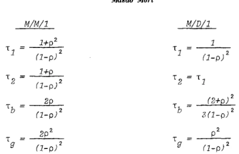
nil

"

_to M/M/1 M/D/1 1+p2 1 '1 _(1-p) 2 '1 2 U-p) '2 = l+p '2 '1 2 (l-p) 'b 2p 'b (2+Q) 2 2 2 (1-p) :3 (1-p) 2p2

,

p2

,

g 2 g _{(1_p)2} (1-p)

Now we transform the number n of the n-th arriving customer into n': for each , and compare the values of y' (= y) numerically for each

n' n

It is notable that the compound ratio '1 : '2 : 'b : 'g is nearly equal

1 : 1 1 : 1 if p is near to 1, but the deviation from this becomes much larger for small p. Thus, for each time transformation,

Y'n'

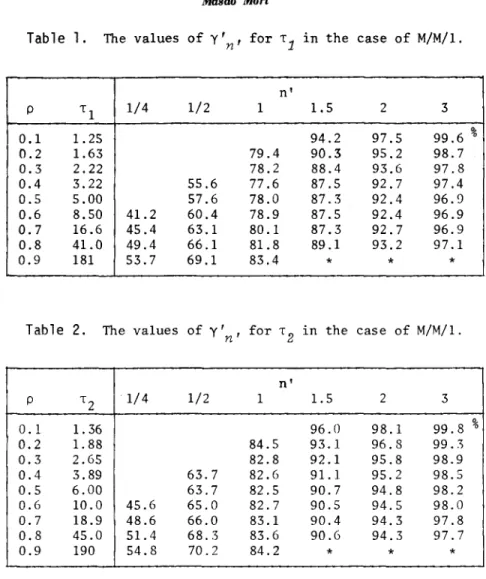
behaves almost similarly in one another when p is near to 1, i.e. when the diffusion approximations are applicable.

Table I and 2 give the values of

Y'n'

which are transformed by '1 and '2 respectively for the case of M/M/I. And Table 3 shows the values of

Y'n'

transformed by '1 (= '2) for the case of M/DIl. The values

Y'n'

in the ta-bles are interpolated linearly by using the exact values of Y for _n

n

=

[n',]

and

n

[n',]

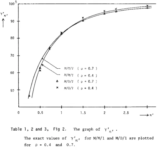
+1. Thus the values in each table may not be so reliable for small n', for Y

n is concave in n. The blanks in the tables are correspond-ing to these unreliable values. In order to avoid this fault, in Figure 2 we plot the exact values of Y_n at n': n/'2 for each n. Nevertheless, the corresponding values in each table seem to be near to one another for every p and n'

,

especially the values in Table 2 and 3 seem to be very near.

Further, in each table, the values of

Y'n'

n' ~ 1/4,

0.1 '\., 0.9).

considered to be almost constant even Hence the time scales and

for every n', excepting varying the value of p (p

can be considered to give fairly nice transformations, and especially '2 may be slightly more favour-able than '1 for p = 0.1 '\., 0.9 and n'> 1/2. ,\nd, when transformed by '2'

Y

2

is about 95% for any p = 0.1 '\., 0.9. lience, in a practical sense, I:e can consider that at n ~ 2'2 the process has almost reached at the equilibrium state.

On the contrary, since the values of 'b and 'g is too small when p is smaller than 0.7 or so, comparing with the values of '1 and '2' the values

Transient Behaviour in M/ M/J and M/ D/J 29

of

Y'n'

transformed by Tb

in Table 1, 2, and 3.

and T does not behave so nicely as the values

g

From the above discussion, the time transformation

n'

=

n/T

2 is

favour-able one both in M/M/l and in M/D/l, but, of course, we cannot apply this re-suIt directly to a general queueing system GI/G/l, even to M/G/l. Thereafter we need exemplify more theoretically on this subj ect.

Acknowledgement

The author wishes to thank Prof. Hidenori Morimura for his guidance and encouragement.

i

100%r---"---~~--! ::

90 80 70 M/l.!/l I.l = 0.7 60 M/M/1 p = 0.4 t. M/D/1 p = 0.7 )( _{M/D/1 p} = 0.4

sa

o

0.5 1.5 2 2.5 ~n'

Table 1, 2 and 3, Fig 2. The graph of y' I

n The exact values of

for p

=

0.4 and

I

Y n' 0.7.

Table 1.

The values of

Y'n'

for '1 in the case of M/M/I. n' p _'1 1/4 1/2 1 1.5 2 3 0.1 1. 25 94.2 97.5 99.6 % 0.2 1.63 79.4 90.3 95.2 98.7 0.3 2.22 78.2 88.4 93.6 97.8 0.4 3.22 55.6 77 .6 87.5 92.7 97.4 0.5 5.00 57.6 78.0 87.3 92.4 96.9 0.6 8.50 41.2 60.4 78.9 87.5 92.4 96.9 0.7 16.6 45.4 63.1 80.1 87.3 92.7 96.9 0.8 41.0 49.4 66.1 81.8 89.1 93.2 97.1 0.9 181 53.7 69.1 83.4 _{* * *}

Table 2.

The values of

Y'n'

for '2 in the case of M/M/I.

n' p _'2 1/4 1/2 1 1.5 2 3 0.1 1. 36 96.0 98.1 99.8 % 0.2 1. 88 84.5 93.1 96.S 99 .. ) 0.3 2.65 82.8 92.1 95.8 98.9 0.4 3.89 63.7 82.6 91.1 95.2 98.5 0.5 6.00 63.7 82.5 90.7 94.8 98.2 0.6 10.0 45.6 65.0 82.7 90.S 94.S 98.0 0.7 18.9 48.6 66.0 83.1 90.4 94.3 97.8 0.8 45.0 51. 4 68.3 83.6 90.6 94.3 97.7 0.9 190 54.8 70.2 84.2 _{* * *}

Table 3.

The values of

Y'n'

for '1 (= '2)

in

the case of M/M/I.

n' p _'2 1/4 1/2 1 1.5 2 3 0.1 1. 23 96.2 98.S 99.3 % 0.2 1. 56 83.7 94.1 97.7 99.4 0.3 2.04 84.4 92.8 96.5 99.1 0.4 2.78 61. 2 82.9 91.7 95.6 98.S 0.5 4.00 42.6 63.3 82.8 91.2 95.2 98.4 0.6 6.25 42.5 64.1 82.6 90.7 94.S 98.2 0.7 11. 1 46.6 65.3 82.8 90.5 94.4 97.9 0.8 25.0 49.5 67.4 83.3 90.5 94.3 97.7 0.9 100 53.9 69.7 84.1 90.7 94.2 *.

Transient Behnviour in Mj Mj 1 and Mj Dj 1

References.

[1] B1omqvist, N., "On the transient behaviour of the GI/G/1 waiting times," Skand. Aktur Tidiskr., (1970), 118-129.

[2] Cohen, J.W., The Single Server Queue, North-Holland, 1969.

.11

[3] Da1ey, D.J., "The serial correlation coefficients of waiting times in a stationary single server queue," J. Austral. Math. Soc., 8 (1968), 683-699. [4J Da1ey, D. J ., "Stochastically monotone Markov Chain," Z. Wahrscheinlichkei

ts-theorie verw. Geb., 10 (1968), 305-317.

[5] Davis, H., "The build-up time of waiting lines," Naval Res. Logist. Quart., 2 (1960), 185-193.

[6] Esary, J.D.F., Proschan, F. and Walkup, D.W., "Association of random vari-ables with applications," Ann. Math. Statist., 38 (1967), 1466-1474. [7] Fell er, ]V., An introduction to probdbU i ty theory and its app lications,

vol. 1, 2nd ed., John Wi1ey, 1957.

[8] Gaver, D.P., "Diffusion approximations and models for certain congestion problems," J. Applied Prob., 5 (1968), 607-623.

[9] Hashida, A., "An evaluation for the rate of convergence to equilibrium state for M/M/s," (in Japanese), reported at Japan OR meeting, Autumn

(1971) .

[10] Heathcote, C.R., "Complete exponential convergence and some related top-ics," J. Applied Prob., 4 (1967), 217-256.

[11] Marchall, K.T., "Some inequalities in queueing," Opns. Res., 16 (1968), 651-658.

[12] Miyazawa, M., "On the rate of convergence of waiting-time distribution," Research Reports on Information Sciences, No. B-1 (1974), (Dept. of Infor-mation Sciences, Tokyo Institute of Technology.)

[13] Morimura, H., "The build-up time of equilibrium waiting time," J. Opns. Res. Soc. Japan, 4 (1962), 76-86.

[14] Newell, G.F., Applications of Queuei~] Theory, Chapman and Hall, 1971. [15] Riordan, J., Combinatorial Identities, John Wi1ey, 1968.

[16] Stoyan, H. and Stoyan, D., "Monotonieeigenschaften der Kundenwartezeiten in Modell GI/G/1," Zeit. Angewandte Mech., 49 (1969), Heft 12, 729-734. [17] Vere-Jones, D., "A rate of convergence problem in the theory of queues,"

Theory Prob. Applications, 9 (1964), 96-103.

Masao MORI

Faculty of Engineering Ibaraki University