Traffic Volum vs. Traveling Distance from the Angle of Operations Research

Journal of the O.R. Society of Japan, Vol. 7, No. 4, May 1965.

TRAFFIC VOLUME VS. TRA VELING DISTANCE FROM THE ANGLE OF OPERATIONS RESEARCH

KUSHIDA YOJI Japan National Railways (Received February 17, 1965)

§ 1. FOREWORD

Traffic volume, when classified as a function of traveling distance, decrease as the latter becomes longer. There have been many attempts over a fairly long period to grasp the quantitative relationship between the traffic volume and the traveling distance. Some, like Mr. G. K. Zipf,

I

say that the traffic volume decrease in inverse to the traveling distance, and others, like Mr. E. C. Young, say that it is inversely proportional to the square of the distance traveled.

The highly developed mechanical civilization of today owes to the remarkable progress of physics. Through physics the laws governing natural phenomena are discovered and expressed numerically and in many cases, it is possible to reproduce the phenomenon many times in a laboratory under conditions arranged as uniformly as possible. On the contray, similar social phenomena might be repeated, but they are some-what different from each other when observed closely. This makes it difficult to grasp the laws in social phenomena with any degree of certainty. The social phenomenon of transportation is no exception. As mentioned previously, there are some people saying that the traffic volume is in inverse proportion to the traveling distance and others who maintain that it is in inverse proportion to the square of the traveling distance. Still others maintain more prudently to vary in inverse proportion in a range somewhat between the first power and the second power. Such different opinions might be ascribable to inadequacies of data, and possibly those holding differing opinions have based these views on different observations.

172

Traffic Volume vs. Traveling Distance 173

A law, which represents something common to individual cases of a social phenomenon taking place under different circumstances, can very often be derived by collecting as much data as possible, because in this way the differences among individual circumstance are averaged out and the factors in common emerge. In this respect, JNR is in a favorable position, having a large body of comprehensive statistics. Owing to such abundant statistical data, it has been possible to make the numerical analyses of traffic volume and traveling distance described below.

§ 2. CASES WHERE EXPONENTIAL DISTRIBUTION GOVERNS

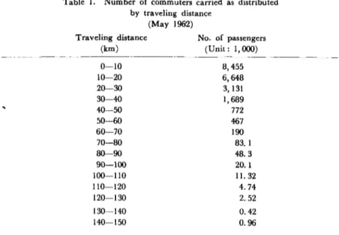
Table I is a frequency distribution of number of commuters carried as a function of traveling distance, calculated by sampling one-tenth of all the 2nd class pass type season tickets for commuters issued by JNR for the month of May 1962. Fig. 1 is its histogram, where the ordinate

--..

---~---Table 1. Number of commuters carried as distributed

by traveling distance (May 1962)

Traveling distance No. of passengers

(km) (Unit: 1, (00) 0-10 8,455 10-20 6,648 20-30 3,131 30-40 1,689 40-50 772 50-60 467 60-70 190 70-80 83.1 80-90 48.3 90-100 20. 1 100-110 11. 32 110-120 4.74 120-130 2.52 130-140 0.42 140-150 0.96

174

.=

.,

..

.,

i

....

Fig. I. Commuter traffic volume by distance of travel

IS III logarithmic scale. In the figure, a broken line runs diagonally. The

fact that this line cuts the upper edges of the columns of traveling distance indicates clearly that this distribution is an exponential one. The number of passengers in the range of less than 10 km in traveling distance stands lower than the broken line. This may be interpreted as showing that a portion of workers are subtracted from short distance railway commuters because they would rather go to work on foot or by bus, in view of the relationship between the distance between their homes and the nearest stations and the distance between their jobs and the nearest station, on the one hand, and the rather small distance of train travel which would

Traffic Volume V8. Traveling Di8tance 175

be involved.

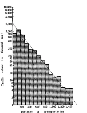
Table 2 and Fig. 2 are the frequency distribution table and the his-togram, respectively, of total tonnage of lumber carried by JNR in 1960, as classified by rail transport distance. It can be said that these data also follow the exponential distribution.

Table 2. Traffic volume of lumber as distributed by distance carriced by rail

(May 1960) Distance of rail shipment

(km) 0-100 100-200 200-300 300-400 400-500 500--600 600-700 700-800 -800-900 900-1,000 1,000-1, lOO 1,100-1,200 1,200-1,300 1,~-I,400 1,400-1,500 Tonnager of lumber (Unit: 1,000 t) 834 1,158 709 333 184 160 99.3 62. I 43.5 17.5 13. I 13.4 4.82 4.29 4.30

Let us give those two propositions a theoretical formula, and compare the figures from the formula with those actually supplied through the statistics. To this end, it is desirable to use the appropriate probability distribution function. The distribution function of the exponential distri-bution is as follows:

F(x)= 1---e-1x _{( 1 )}

. This can be restated as:

(2) It means that the ratios of the cumulative totals made up by adding

176 10,000 8.000 6,000 Yoji KU8hida Distance of transportation

Fig. 2. Traffic volume of lumber by distance of transportation

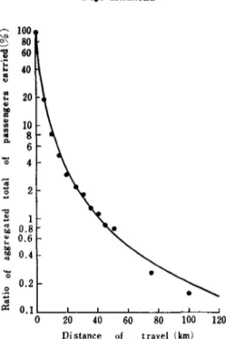
values of x, in order from large to small, follow the exponential function. To explain this using the example of commuters' traffic cited before, Table 3 and Fig. 3 will be used. The relation between the calculated values in Table 3 and the straight line Fig. 3 is expressed by the follow-ing equation:

W(X)= 125e-O•071,1' (3)

Taking the example of transportation of commuters and lumber, it has become clear that the traffic volume is distributed exponentially with respect to distance of transportation. But the question remains as to whether this is the only observable phase of the traffic phenomena of passenger transportation and goods transportation.

Traffic Volume v.. Traveling D;.tance 177 Table 3. Total commuter traffic as distributed by traveling distance (May 1962) Trave1ing distance Total no. of passengers Ratio Calculated value W(.~)

... (km) (Unit: 1,000 psrs). (%) (%) o 21,524 100 125 10 13,069 60.7 61. 5 20 6,421 29.8 30.3 30 3,290 15.3 14.9 40 1,601 7.44 7.33 50 829 3.85 3.61 60 362 1. 68 I. 77 70 172 O. 798 O. 876 80 88.9 0.413 0.431 90 40.6 O. 189 0.212 100 20.5 0.095 0.104 1 \0 9.18 0.043 0.051 120 4.44 0.021 0.025 130 1. 92 0.009 0.012 140 1. 50 O. 006 O. 006 over 150 0.50 0.003 0.003 100 80 ~ 60

'"

..

'"

-

"

"

....

....

'"

a

'"

..

.,

....

·z

_.,

178 Yoji KU6hida

§ 3. CASES WHERE HYPER-EXPONENTIAL DISTRIBUTION GOVERNS

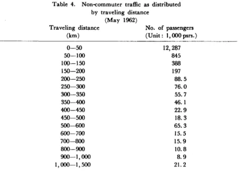
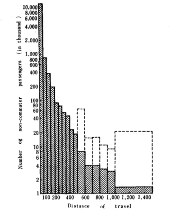
Table 4 and Fig. 4 were worked out by sampling one-tenth of the 2nd class non-commuter passengers carried by JNR in May 1962. One is the frequency distribution and the other is its histogram, of number of pas-sengers grouped by traveling distance. As the statistical data are not grouped in equal ranges of traveling distance, the columns of 100 km and 500 km range in Fig 4 are shown by dotted lines. As can be easily inferred from the figure, the traffic in this case does not seem to follow the ex-ponential distribution.

Table 4. Non-commuter traffic as distributed by traveling distance

(May 1962)

Traveling distance No. of passengers

(km) (Unit: 1,000 psrs.) 0-50 12,287 50-100 845 100-150 388 150-200 197 200-250 88.5 250-300 76.0 300-350 55. 7 350-400 46.1 400-450 22.9 450-500 18.3 500-600 65.3 600-700 15.5 700-800 15.9 800-900 10.8 900-1,000 8.9 1,000-1,500 21. 2

For commuters, it may be understood that there is little effect, in view of their purpose of travel, of the cost of travel (in time, effort and money, in relation to their gains from the transport. For long-distance

Traffic Volume vs. Traveling Distance 179

..,

..

"

'"

...

""

_..

...

...

-

_"

""

...

.,

"

Fig. 4. Non-commuter traffic volume by distance of travel

travelers, however, the cost of travel to the passenger can be regarded as proportional to the traveling distance. Therefore, the average traveling distance, which is deemed to represent the balance between their gains from and their costs of travel, may be rightly taken as a single quantity. The inversion of such an average traveling distance is shown as ,( in equation (1) and (2).

The aims of traffic by non-commuters vary greatly. Passengers for shopping are concerned about small sacrifices for their short distance riding, while sightseeing passengers are less likely to mind a considerable long travel distance. Therefore it is unreasonable to have and approach

180 Y oji KU8laida

to the problem of non-commuter passengers merely through the one ave-rage traveling distance as was done in the case of commuters. Traffic analysis in this regard, it may be considered, 'should involve different values of average traveling distance varying with the aim of riding. In other words, it becomes necessary to introduce another concept of distribu-tion which is extended from the exponential distribudistribu-tion. To this end a distribution compounding the exponential distribution and Pearson's III-type distribution is considered. This, in construction, may be regarded as a kind of hyper-exponential distribution. Its distribution function is given below:

(4)

Then, let us examine the case where a in equation (4) takes a parti-cular value:

When a=oo, equation (4) will turn to equation (1), which represents an ordinary exponential distribution.

When a= 1, equation (4) will become the following:.

1

F ( x ) = l

-I+Aox This will be modified as:

~=l-F(x)

X+-AO

(5)

(6)

Equations (5) or (6), indeed, are the prototypes of formulas applicable to non-commuter passengers. The explanations of why the actual values for commuters for a very short distance deviate from the theoretical dis-tribution applies to the non-commuters in much the same way. There is also a good reason for the values of non-commu,ter passengers to deviate from the theoretical distribution in the case of a very long distance as

Traffic Volume VB. Traveling DiBtance 181

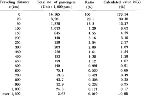
well. This is because the railway routes are limited and the distribution of population cannot be said to be uniform throughout the country in-cluding remote areas. Form such considerations the equation is modified a little, and then the calculated values are compared with the actual statistics. The result is shown in Table 5 and Fig. 5. The theoretical values in Table 5 and the curve in Fig- 5 are the result of the following equation:

751

W(x)= x+4. 24~-O. 58

(7)

When the relation between traffic volume and traveling distance is considered, one aspect of the problem is the expected traffic volume for a certain traveling distance. This it determined from the probability density for a given distance of transportation. From equation (5), the

Table 5. Total non-commuter traffic as distributed by traveJing distance (May 1962)

TraveJing distance Total no. of passengers Ratio Calculated value W(x)

x (km) (Unit: 1,000psrs.) (%) (%) 0 14.165 100 176.54 20 3,981 28. 1 30.40 50 1,878 13.3 13.27 100 1,033 7.29 6.62 150 645 4.55 4.29 200 448 3.16 3. \0 250 359 2.54 2.37 300 283 2.00 1. 89 350 228 1. 61 1. 54 400 182 1. 28 1. 28 450 159 1. 12 1. 07 500 140 0.991 0.91 600 75. 1 0.530 0.66 700 59.6 0.421 0.49 800 43. 7 0.308 0.35 900 32.9 0.232 0.25 1,000 24.3 0.171 0.17 over 1,500 2.67 0.019 -0.08

182

....

_...

..

"

...

..

j

"

.

..

2

....

..

...

_..

Fig. 5. Aggregated total of non-commuter traffic by distance of travel

probability density is:

f(x) (8 )

The value of

-.L

small that the traffic volume can be said to decrease in inverse proportion to the square of the transportation distance if the distance x is long enough, according to evuation (8). In fact, taking the values in Fig. 4 for the range of transportation distance from 100 to 500 km, it may be correct to say that the traffic volume is in inverse proportion to the square of the transportation distance. However, this should not lead to the hasty conclusion that the traffic phenomenon also is governed by the well-known inverse square law of physical phenomena.

Traffic· Volume V8. Traveling Di8tance 183

There are some cases as mentioned above, such as commuter traffic, which follow the exponential distribution. Furtla.ermore, there are some other situations in which traffic does not vary ~n inverse proportion to the square of the distance, as seen in the example cited below.

§ 4. CASES OF COMMERCIAL AUTOMOBILES

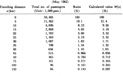
Table 6 and Fig. 6 give actual figures obtained in the survey on commercial automobiles for the month of October 1960, and the cor-responding values calculated by equation (9) set down below which is considered theoretically adoptable in this case:

W 1,393

(x)= (X+4)1.9 (9)

Equation (9) corresponds to a modified equation (4) with 1. 9 substitut-ing for a. To indicate it as a probability density function as before, the traffic volume is seen decreasing in inverse proportion to the 2. 9th power

Table 6. Total traffic by commercial motorcars as distributed by traveling distance

(May 1962)

Traveling distance Total no. of passengers Ratio Calculated value W(x)

x(km) (Unit: 1,000 psrs.) (%) (%) 0 59,485 lOO lOO 5 1l,362 19. I 21. 4 10 4,896 8.23 9.26 15 2,868 4.82 5. 18 20 1,783 3.00 3.32 25 1,303 2. 19 2.32 30 1,087 1. 83 1. 71 35 798 1. 34 1. 32 40 656 1.10 1. 05 45 515 0.866 0.856 50 465

o.

1114 Yoji KUlJhida ~ ₁₀₀ ~

_...

..

..

•

..

..

"

..

..

""

-

'"

..

...

....

-

•

Fig. 6. Aggregated traffic volume of commercial passenger motor cars by distance of travel

of the sum of the traveling distance 4 km. Roughly speaking, the traffic volume here decreases in inverse proportion to about the 3rd power of the traveling distance.

The purpose of operations research is to assist the executive and other managerial members at various levels of business organization so that they may be able to make the best decision on many complicated pro-blems the enterprise encounters in carrying on operation. To this end it is necessary to take a scientific approach to the problem, where the mathe-matical method is given primary importance. The proposition taken up in this article is not the sort of subject which is of direct use for manage-ment decision, and as such it might not be said to be OR.

JNR has very comprehensive statical data. These statistical data are valuable materials derived through surveys. They contain material of immeasurable potential value.

Traffic· Volume vs. Traveling Distance 185 As seen in Fig. 3, the frequency distribution of commuter passengers well conforms to the exponential distribution in the range from 60% to 0.06%, i.e. to the extent where the figures are of three digits. Such a clear cut example will not be found anywhere else. In other words, all this tells how valuable JNR's data are, in that such an adequate number of values are obtained in the survey. It would be wasteful to do nothing better than statistical handing with such precious materials. However short of capacity we may find ourselves, this is where we must be con-scious of our duty of tackling problems as they challenge us.