Multivariate normality test using Srivastava's skewness and kurtosis

Multivariate normality test using Srivastava’s

skewness and kurtosis

Rie Enomoto, Naoya Okamoto and Takashi Seo

(Received March 6, 2012; Revised June 15, 2012)

Abstract. In this paper, we consider the multivariate normality test based on the sample measures of multivariate skewness and kurtosis defined by Srivas-tava [11]. Koizumi et al. [4] proposed test statistics M1 and M2 using Srivas-tava’s sample skewness and kurtosis, which are asymptotically distributed as

χ2-distribution. We propose a new test statistic M3 by taking account of the variance of M2 under the normality. In order to evaluate the accuracy of the proposed test statistic, the numerical results by a Monte Carlo simulation for some selected values of parameters are presented.

AMS 2010 Mathematics Subject Classification. 62E20, 62H10, 65C05.

Key words and phrases. Multivariate skewness, multivariate kurtosis,

Jarque-Bera test, test for multivariate normality.

§1. Introduction

In statistical analysis, the test for normality is an important problem. This problem has been considered by many authors. For the univariate case, the test statistic using order statistic derived by Shapiro and Wilk [10] is one of the most famous and essential tests for normality. Another approach for testing normality uses sample skewness and kurtosis separately. D’Agostino [2] derived the test statistic using sample skewness. For the test statistic using sample kurtosis, Anscombe and Glynn [1] proposed the test statistic distributed as standard normal distribution. Jarque and Bera [3] proposed the bivariate test using univariate sample skewness and kurtosis. The improved Jarque-Bera (JB) test statistics have been considered by many authors (see, e.g. Urz´ua [12] and Nakagawa et al. [5]).

Mardia [6] and Srivastava [11] gave different definitions of multivariate sam-ple skewness and kurtosis, and discussed some test statistics using these mea-sures for assessing multivariate normality. Mardia and Foster [7] proposed

the test statistics using Mardia’s sample skewness and kurtosis. Okamoto and Seo [8] derived the improved approximate χ2 test statistic using multivariate sample skewness of Srivastava [11], which is more accurate than Srivastava’s

χ2 test statistic. The test statistics using the multivariate sample kurtosis of Srivastava [11] were discussed by Seo and Ariga [9]. The test statistics M1and

M2 using Srivastava’s sample skewness and kurtosis that are asymptotically distributed as χ2-distribution were proposed by Koizumi et al. [4]. However, for a small N , there is difference between the upper percentiles of distributions of their statistics and the χ2-distribution. Thus, it seems that the multivariate normality test based on M1 or M2, though applicable, is not appropriate. Our purpose is to propose a new test statistic M3 by taking account of the variance of M2 under the normality. We investigate the accuracies of variances, upper percentiles, type I errors and powers for the multivariate JB test statistics M1,

M2 and M3 via a Monte Carlo simulation for selected values of parameters.

§2. Srivastava’s measures of multivariate skewness and kurtosis

Let x be a p-dimensional random vector with mean vector µ and covariance matrix Σ = ΓDλΓ0, where Γ = (γ1, γ2, . . . , γp) is an orthogonal matrix and Dλ = diag(λ1, λ2, . . . , λp). Note that λ1, λ2, . . . , λp are the eigenvalues of Σ.

Then, Srivastava [11] defined the population measures of multivariate skewness and kurtosis as β_1,p2 = 1 p p ∑ i=1 { E[(yi− θi)3] λ 3 2 i }2 , β2,p= 1 p p ∑ i=1 E[(yi− θi)4] λ2_i ,

respectively, where yi = γ0ix and θi = γ0iµ (i = 1, 2, . . . , p). We note that β_1,p2 = 0, β2,p = 3 under a multivariate normal population.

Let x1, x2, . . . , xN be samples of size N from a multivariate population. Let x and S = HDωH0 be the sample mean vector and sample covariance

matrix given as x = 1 N N ∑ j=1 xj, S = 1 N N ∑ j=1 (xj− x)(xj− x)0,

respectively, where H = (h1, h2, . . . , hp) is an orthogonal matrix and Dω =

diag (ω1, ω2, . . . , ωp). We note that

ωi= h0_iShi= 1 N N ∑ j=1 (yij − yi)2, i = 1, 2, . . . , p, where yij = h0ixj (i = 1, 2, . . . , p, j = 1, 2, . . . , N ), yi = N−1 ∑N j=1yij (i =

1, 2, . . . , p). Then, Srivastava [11] defined the sample measures of multivariate skewness and kurtosis as

b2_1,p =1 p p ∑ i=1 { 1 ω 3 2 i N ∑ j=1 (yij − yi)3 N }2 = 1 p p ∑ i=1 { m3i m 3 2 2i }2 , b2,p = 1 p p ∑ i=1 1 ω2 i N ∑ j=1 (yij − yi)4 N = 1 p p ∑ i=1 m4i m2 2i ,

respectively, where mνi = N−1

∑N

j=1(yij− yi)ν.

Koizumi et al. [4] proposed two test statistics for multivariate normality:

M1 = N p { b2_1,p 6 + (b2,p− 3)2 24 } d − → χ2 p+1, M2 = pb2_1,p E[b2 1,p] +(b2,p− E[b2,p]) 2 Var[b2,p] d − → χ2 p+1

for large N , where the expectation of b2

1,p, and the expectation and variance of b2,p are given by E[b2_1,p]; 6(N− 2) (N + 1)(N + 3), E[b2,p]; 3(N − 1) N + 1 , Var[b2,p]; 24N (N − 2)(N − 3) p(N + 1)2_{(N + 3)(N + 5)},

respectively under the normality.

§3. New multivariate JB test statistic using the variance of M2 The test statistic M2 was introduced in Koizumi et al. [4] so that the accuracy of the upper percentile for the approximate test statistic is better than that of the test statistic M1 for small N . However, for a small N , it seems that there

is difference between the the upper percentiles of the distributions of M2 and the χ2-distribution. Hence, we propose a new test statistic to be closer to the upper percentile of the χ2-distribution by using the variance of M2. The idea of our proposal of M3 is that E[M3] = p + 1 and Var[M3] = 2(p + 1).

Theorem 1. For a large N , the test statistic M3

M3 = cM2+ (1− c)(p + 1)

is asymptotically distributed as a χ2_p+1-distribution, where

c = { 2(p + 1) Var[M2] }1 2 .

In Appendix, Var[M2] will be derived under the normality, as follows: Var[M2]; 2 pN (N − 2)(N − 3)(N + 5)(N + 7)(N + 9)(N + 11)(N + 13) ×{p(p + 1)N8+ 2(29p2+ 110p + 135)N7 +(859p2+ 3055p + 702)N6+ 2(1058p2− 217p − 7272)N5 −(21665p2_{+ 71105p + 38844)N}4 −2(13471p2_{+ 10792p− 96183)N}3 +3(44759p2+ 130587p + 134898)N2+ 90(767p− 6222)N +81000}(N 6= 2, 3). (3.1) §4. Simulation studies

The accuracies of variances, upper percentiles, type I errors and powers of the multivariate JB test statistics M1, M2 and M3 are evaluated via a Monte Carlo simulation study. Simulation parameters are as follows: p = 3, 10, 20, 30; N = 20, 50, 100, 200, 400, 800 (p < N ); and significance level α = 0.05. As a numerical experiment, we carry out 1,000,000 replications.

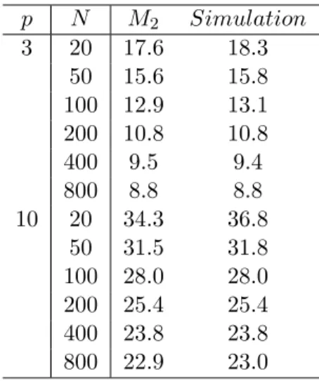
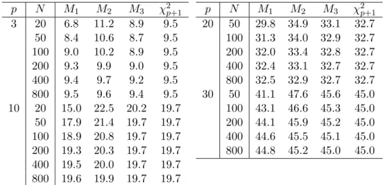
First, we compare variance (3.1) with simulated variances derived by Monte Carlo simulation. In Table 1, “M2” denotes values calculated using (3.1). M2 and simulated values are almost the same for all parameters. Next, we check Var[M3] = 2(p + 1). In Table 2, “M3” represents variance Var[M3] = 2(p + 1) and “Simulation” is simulated variance of the test statistic M3 derived by Monte Carlo simulation. It can be seen from Table 2 that M3 has almost the same variance as the χ2_p+1-distribution for all parameters. Table 3 gives the values of the upper 5 percentiles of M1, M2 and M3. When N is small, they show that difference between M3 and χ2_p+1-distribution is smaller than

that between χ2_p+1-distribution and M2. Table 4 gives the values of type I errors of M1, M2 and M3. They show that M3 is closer to 0.05 than others when N is small. We note that if type I error is smaller than 0.05, the test is conservative. M1 is always conservative and M2is not conservative. M3is not conservative and the approximate accuracy of M3 is outstanding except when

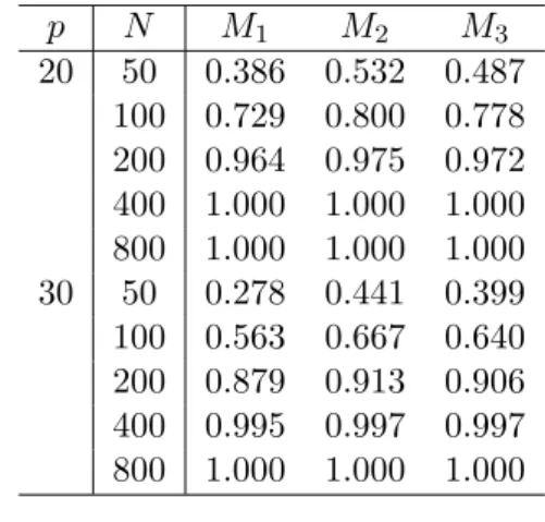
p is small. Table 5 gives the values of the powers of M1, M2 and M3, where each element of the sample is generated using χ2₅-distribution. The power of

M2 is the highest. Although Laplace distribution, lognormal distribution and beta distribution are also used as samples, the same tendency was seen.

In conclusion, the simulation results indicate that M3 has almost the same variance and the upper 5 percentile as the χ2_p+1-distribution even for a small sample size. Although the test statistic M2 may have the best power, type I error of M2 has far exceeded 0.05 for a small sample size. In addition, the upper 5 percentile of M3 is the closest to that of χ2_p+1-distribution for a small sample size. Therefore, the multivariate JB test statistic M3 proposed in this paper is useful for the multivariate normality test.

§A. Derivation of (3.1)

In this appendix, we calculate variance Var[M2] as follows: Var[M2] = Var[T1] + Var[T2] + 2Cov[T1, T2], where T1 = pb2_1,p E[b2 1,p] , T2 = (b2,p− E[b2,p])2 Var[b2,p] .

Now, we derive the moments under the hypothesis that x1, . . . , xN are i.i.d. from Np(µ, Σ). For large N , we get

yij = h0_ixj −→ N(γd 0iµ, λi)

because hi → γi with probability one (see Srivastava [11]). Thus, yi1, yi2, . . . , yiN are asymptotically independently normally distributed. Further, the fol-lowing expression was described by Srivastava [11] for large N .

E[mk_νim−νk/2_2i ]E[mνk/2_2i ]; E[mk_νi].

We checked the above equation numerically. In order to simplify calculation of a moment, dependence of yij and yi is avoided as follows. Let y

(α)

i be a

mean defined on the subset of yi1, yi2, . . . , yiN, that is,

y(α)_i = 1 N− 1 N ∑ j=1,j6=α yij.

Then, yiα is asymptotically independent of y(α)_i . Without a loss of generality,

we calculate the moments with µ = 0 and λi = 1, that is, Σ = I, because b21,p and b2,p are hardly influenced by Σ for a large N . In addition, we put

y(α)_i = √ 1

N − 1Zi.

Since Zi is distributed as a standard normal distribution for large N , the odd

order moments approximately equal zero for calculating moments and

E[Z_i2k]; (2k − 1) · · · 5 · 3 · 1, k = 1, 2, . . . . We note that Var[T1] = p2 (E[b2_1,p])2Var[b 2 1,p], Var[T2] = 1 (Var[b2,p])2 [

E[b4_2,p]− 4E[b2,p]E[b3_2,p] +E[b2_2,p]{8(E[b2,p])2− E[b22,p]

} − 4(E[b2,p])4 ] , Cov[T1, T2] = p E[b2_1,p]Var[b2,p] {

Cov[b2_1,p, b2_2,p]− 2E[b2,p]Cov[b2_1,p, b2,p]},

where

Cov[b2_1,p, b2,p] = E[b21,pb2,p]− E[b21,p]E[b2,p], Cov[b2_1,p, b2_2,p] = E[b2_1,pb2_2,p]− E[b2_1,p]E[b2_2,p].

Since Okamoto and Seo [8] derived Var[b2_1,p], we have only to derive the mo-ments E[b3_2,p], E[b4_2,p], E[b2_1,pb2,p] and E[b21,pb22,p] under the normality.

Now, we consider the expectation E[b3_2,p]. We have

E[b3_2,p] = E [{ 1 p p ∑ i=1 m4i m2 2i }3] = 1 p3 { ∑ i E [ m3_4i m6 2i ] +∑ i6=j E [ m2_4im4j m4 2im22j ] + ∑ i6=j6=k6=i E [ m4im4jm4k m2 2im22jm22k ]} ,

where E[m4i] = ( 1− 1 N )4 E[C_iα4 ], E[m2_4i] = 1 N2 ( 1− 1 N )8_{

N E[C_iα8 ] + N (N− 1)E[C_iα4 C_iβ4 ] } , E[m3_4i] = 1 N3 ( 1− 1 N )12_{

N E[C_iα12] + 3N (N − 1)E[C_iα8 C_iβ4 ] +N (N − 1)(N − 2)E[C_iα4 C_iβ4 C_iγ4]

} , E[m2_2i] = 1 N2 ( 1− 1 N )4_{

N E[C_iα4 ] + N (N− 1)E[C_iα2 C_iβ2 ] } , E[m4_2i] = 1 N4 ( 1− 1 N )8_{

N E[C_iα8 ] + 4N (N− 1)E[C_iα6 C_iβ2]

+3N (N − 1)E[C_iα4 C_iβ4] + 6N (N − 1)(N − 2)E[C_iα4 C_iβ2 C_iγ2] +N (N − 1)(N − 2)(N − 3)E[C_iα2 C_iβ2 C_iγ2C_iδ2]

} , E[m6_2i] = 1 N6 ( 1− 1 N )12_{

N E[C_iα12] + 6N (N − 1)E[C_iα10C_iβ2]

+15N (N− 1)E[C_iα8 C_iβ4] + 15N (N − 1)(N − 2)E[C_iα8 C_iβ2 C_iγ2] +10N (N− 1)E[C_iα6 C_iβ6] + 60N (N − 1)(N − 2)E[C_iα6 C_iβ4 C_iγ2] +20N (N− 1)(N − 2)(N − 3)E[C_iα6 C_iβ2 C_iγ2C_iδ2]

+15N (N− 1)(N − 2)E[C_iα4 C_iβ4C_iγ4]

+45N (N− 1)(N − 2)(N − 3)E[C_iα4 C_iβ4 C_iγ2C_iδ2]

+15N (N− 1)(N − 2)(N − 3)(N − 4)E[C_iα4 C_iβ2 C_iγ2C_iδ2C_i²2] +N (N − 1)(N − 2)(N − 3)(N − 4)(N − 5)

×E[C2

iαCiβ2Ciγ2Ciδ2Ci²2Ciζ2]

}

, (α, β, γ, δ, ², ζ are all distinct)

and Ciα = yiα − y(α)_i . It is easy to calculate them because yiα and y(α)_i are

After extensive calculations, we obtain E[m4i]; 3(N− 1) 2 N2 , E[m2_4i]; 3(N− 1)(3N 3_{+ 23N}2_{− 63N + 45)} N4 , E[m3_4i]; 27(N− 1)(N 5_{+ 27N}4_{+ 226N}3_{− 1098N}2_{+ 1725N− 945)} N6 , E[m2_2i]; (N− 1)(N + 1) N2 , E[m4_2i]; (N− 1)(N + 1)(N + 3)(N + 5) N4 , E[m6_2i]; (N− 1)(N + 1)(N + 3)(N + 5)(N + 7)(N + 9) N6 ,

and we can obtain the expectation for b3_2,p as

E[b3_2,p]; 27{p2N7+ p(21p + 8)N6+ (137p2+ 80p + 64)N5

+(197p2− 176p − 640)N4− (693p2+ 1664p− 2112)N3

−(809p2_{− 4776p + 2560)N}2_{+ 3(697p}2_{− 1008p + 256)N}

−945p2}_× 1

p2_{(N + 1)}3_{(N + 3)(N + 5)(N + 7)(N + 9)}.

Similarly, we get the expectations E[b4_2,p], E[b2_1,pb2,p] and E[b2_1,pb2_2,p] as follows:

E[b4_2,p]; 27 p3 { 3p3N12+ 12p2(13p + 4)N11 +2p(1659p2+ 984p + 416)N10 +12(3069p3+ 2424p2+ 1504p + 960)N9 +(221565p3+ 165312p2+ 46016p− 85248)N8 +8(78663p3− 3996p2− 105568p − 34368)N7 +12(6687p3− 276552p2− 155312p + 249984)N6 −8(435261p3_{+ 584736p}2_{− 1781584p + 278496)N}5 −3(1164721p3_{− 7721536p}2_{− 2766528p + 7525120)N}4 +12(770105p3+ 1570500p2− 7438208p + 4324608)N3 +18(330851p3− 4060968p2+ 5142144p− 1830912)N2 −540(28283p3_{− 72072p}2_{+ 36608p− 7680)N + 6081075p}3} × 1 (N + 1)4_{(N + 3)}2_{(N + 5)}2_{(N + 7)(N + 9)(N + 11)(N + 13)},

E[b2_1,pb2,p]; 18(N− 2){pN3+ (11p + 12)N2+ (23p− 36)N − 35p} p(N + 1)2_{(N + 3)(N + 5)(N + 7)} , E[b2_1,pb2_2,p]; 18(N− 2) p2_{(N + 1)}3_{(N + 3)}2_{(N + 5)(N + 7)(N + 9)(N + 11)} ×{3p2N7+ p(99p + 80)N6+ (1203p2+ 1544p + 1440)N5 +(6315p2+ 5920p− 6048)N4 +(10737p2− 22160p − 12768)N3 −3(4853p2_{+ 22480p− 20704)N}2 −9(3887p2_{− 10824p + 2752)N + 31185p}2}_. Thus, we can obtain

Var[T1]; 6N (N3+ 37N2+ 11N− 313) (N − 2)(N + 5)(N + 7)(N + 9) (see [8]), Var[T2]; 2(N + 1)2(N5+ 123N4− 67N3− 2667N2+ 4842N + 5400) N (N − 2)(N − 3)(N + 7)(N + 9)(N + 11)(N + 13) , Cov[b2_1,p, b2,p]; 216N (N − 2)(N − 3) p(N + 1)2_{(N + 3)(N + 5)(N + 7)}, Cov[b2_1,p, b2_2,p]; 432N (N − 2)(N − 3) p2_{(N + 1)}3_{(N + 3)}2_{(N + 5)(N + 7)(N + 9)(N + 11)} ×{3pN4+ 6(11p + 10)N3+ 24(17p− 3)N2 +2(207p− 374)N − 891p + 344}, Cov[T1, T2]; 12(15N3− 18N2− 187N + 86) (N − 2)(N + 7)(N + 9)(N + 11), which yield (3.1). Acknowledgements

The authors would like to thank the referee for his useful comments. Any re-maining errors are the authors’ responsibility. The research of the third author was supported in part by Grant-in-Aid for Scientific Research (C) (23500360).

Table 1: Variance of M2. p N M2 Simulation 3 20 17.6 18.3 50 15.6 15.8 100 12.9 13.1 200 10.8 10.8 400 9.5 9.4 800 8.8 8.8 10 20 34.3 36.8 50 31.5 31.8 100 28.0 28.0 200 25.4 25.4 400 23.8 23.8 800 22.9 23.0 p N M2 Simulation 20 50 55.8 56.4 100 50.7 50.7 200 46.9 46.8 400 44.6 44.7 800 43.3 43.4 30 50 80.2 81.6 100 73.5 73.6 200 68.5 68.5 400 65.4 65.5 800 63.8 63.7 Table 2: Variance of M3. p N M3 Simulation 3 20 8.0 8.3 50 8.0 8.1 100 8.0 8.1 200 8.0 8.0 400 8.0 7.9 800 8.0 8.0 10 20 22.0 23.6 50 22.0 22.2 100 22.0 22.0 200 22.0 22.0 400 22.0 22.0 800 22.0 22.0 p N M3 Simulation 20 50 42.0 42.5 100 42.0 42.1 200 42.0 41.9 400 42.0 42.0 800 42.0 42.0 30 50 62.0 63.1 100 62.0 62.1 200 62.0 62.1 400 62.0 62.0 800 62.0 61.9

Table 3: The upper 5 percentiles of M1, M2 and M3. p N M1 M2 M3 χ2p+1 3 20 6.8 11.2 8.9 9.5 50 8.4 10.6 8.7 9.5 100 9.0 10.2 8.9 9.5 200 9.3 9.9 9.0 9.5 400 9.4 9.7 9.2 9.5 800 9.5 9.6 9.4 9.5 10 20 15.0 22.5 20.2 19.7 50 17.9 21.4 19.7 19.7 100 18.9 20.8 19.7 19.7 200 19.3 20.3 19.7 19.7 400 19.5 20.0 19.7 19.7 800 19.6 19.9 19.7 19.7 p N M1 M2 M3 χ2p+1 20 50 29.8 34.9 33.1 32.7 100 31.3 34.0 32.9 32.7 200 32.0 33.4 32.8 32.7 400 32.4 33.1 32.7 32.7 800 32.5 32.9 32.7 32.7 30 50 41.1 47.6 45.6 45.0 100 43.1 46.6 45.3 45.0 200 44.1 45.9 45.2 45.0 400 44.6 45.5 45.1 45.0 800 44.8 45.2 45.0 45.0

Table 4: Type I errors of M1, M2 and M3.

p N M1 M2 M3 3 20 0.021 0.070 0.042 50 0.037 0.064 0.040 100 0.043 0.060 0.041 200 0.046 0.056 0.043 400 0.048 0.054 0.045 800 0.050 0.053 0.048 10 20 0.013 0.079 0.055 50 0.032 0.070 0.050 100 0.041 0.064 0.050 200 0.046 0.058 0.050 400 0.048 0.055 0.050 800 0.049 0.053 0.050 p N M1 M2 M3 20 50 0.027 0.072 0.054 100 0.037 0.064 0.052 200 0.043 0.058 0.051 400 0.047 0.055 0.051 800 0.048 0.053 0.051 30 50 0.023 0.072 0.055 100 0.035 0.064 0.053 200 0.042 0.059 0.052 400 0.046 0.055 0.051 800 0.048 0.052 0.050

Table 5: Powers of M1, M2 and M3. p N M1 M2 M3 3 20 0.264 0.414 0.331 50 0.756 0.805 0.742 100 0.960 0.967 0.954 200 0.998 0.998 0.998 400 1.000 1.000 1.000 800 1.000 1.000 1.000 10 20 0.154 0.349 0.294 50 0.586 0.690 0.645 100 0.903 0.929 0.916 200 0.995 0.997 0.996 400 1.000 1.000 1.000 800 1.000 1.000 1.000 p N M1 M2 M3 20 50 0.386 0.532 0.487 100 0.729 0.800 0.778 200 0.964 0.975 0.972 400 1.000 1.000 1.000 800 1.000 1.000 1.000 30 50 0.278 0.441 0.399 100 0.563 0.667 0.640 200 0.879 0.913 0.906 400 0.995 0.997 0.997 800 1.000 1.000 1.000 References

[1] F. J. Anscombe and W. J. Glynn, Distribution of the kurtosis statistic b2 for

normal samples, Biometrika 70 (1) (1983), 227–234.

[2] R. B. D’Agostino, An omnibus test of normality for moderate and large size

samples, Biometrika 58 (1971), 341–348.

[3] C. M. Jarque and A. K. Bera, A test for normality of observations and regression

residuals, International Statistical Review 55 (1987), 163–172.

[4] K. Koizumi, N. Okamoto and T. Seo, On Jarque-Bera tests for assessing

multi-variate normality, Journal of Statistics: Advances in Theory and Applications 1

(2009), 207–220.

[5] S. Nakagawa, H. Hashiguchi and N. Niki, Improved omnibus test statistic for

normality, Computational Statistics 27 (2012), 299–317.

[6] K. V. Mardia, Measures of multivariate skewness and kurtosis with applications, Biometrika 57 (1970), 519–530.

[7] K. V. Mardia and K. Foster, Omnibus tests of multinormality based on skewness

and kurtosis, Communications in Statistics–Theory and Methods 12 (1983), 207–

221.

[8] N. Okamoto and T. Seo, On the distributions of multivariate sample skewness, Journal of Statistical Planning and Inference 140 (2010), 2809–2816.

[9] T. Seo and M. Ariga, On the distribution of kurtosis test for multivariate

nor-mality, Journal of Combinatorics, Information & System Sciences 36 (2011),

[10] S. S. Shapiro and M. B. Wilk, An analysis of variance test for normality

(com-plete samples), Biometrika 52 (1965), 591–611.

[11] M. S. Srivastava, A measure of skewness and kurtosis and a graphical method

for assessing multivariate normality, Statistics & Probability Letters 2 (1984),

263–267.

[12] C. M. Urz´ua, On the correct use of omnibus tests for normality, Economic Letters

53 (1996), 247–251.

Rie Enomoto

Department of Mathematical Information Science, Tokyo University of Science 1-3 Kagurazaka, Shinjuku-ku, Tokyo 162-8601, Japan

E-mail : [email protected]

Naoya Okamoto

Department of Food Sciences, Tokyo Seiei College

1-4-6 Nishishinkoiwa, Katsushika-ku, Tokyo 124-8530, Japan

E-mail : n [email protected]

Takashi Seo

Department of Mathematical Information Science, Tokyo University of Science 1-3 Kagurazaka, Shinjuku-ku, Tokyo 162-8601, Japan