A GPU Implementation of a Bit-parallel Algorithm for Computing Longest Common Subsequence

全文

(1)Vol.2014-MPS-97 No.12 2014/3/3. IPSJ SIG Technical Report. A GPU Implementation of a Bit-parallel Algorithm for Computing Longest Common Subsequence Katsuya Kawanami1,a). Noriyuki Fujimoto1,b). Abstract: The longest common subsequence (LCS for short) for given two strings has various applications, e.g. com-. parison of DNAs. In the paper, we propose a GPU algorithm to accelerate Hirschberg’s LCS algorithm improved with Crochemore et al.’s bit-parallel algorithm. Crochemore et al.’s algorithm includes bitwise logical operators, which can be easily computed in parallel because they have bitwise parallelism. However, Crochemore et al.’s algorithm also includes an operator with less parallelism, i.e. an arithmetic sum. In the paper, we focus on how to implement these operators efficiently in parallel and experimentally show the following results. First, the proposed GPU algorithm with 2.67 GHz Intel Core i7 920 CPU and GeForce GTX 580 GPU runs maximum 15.14 times faster than the bit-parallel CPU algorithm using a single core with 2.67 GHz Intel Xeon X5550 CPU. Next, the proposed GPU algorithm runs maximum 4.09 times faster than the bit-parallel CPU algorithm using four cores with 2.67 GHz Intel Xeon X5550 CPU. Furthermore, the proposed algorithm with GeForce 8800 GTX runs 10.9 to 18.1 times faster than Kloetzli et al.’s existing GPU algorithm with the same GPU. Keywords: Longest Common Subsequence(LCS), bit-parallel algorithm, GPGPU. 1. Introduction There are various metrics of the similarity between two strings, for example, the edit distance. The longest common subsequence [6] (LCS for short) is one of them. LCS can be applied to various problems, e.g. comparison of DNAs, inexact string matching, spell checking, and others. When the lengths of given two strings are m and n, one of the LCSs can be computed by dynamic programming in O(mn) time and O(mn) space [7]. However, m and n can be huge for comparison of DNAs. So, O(mn) space is not acceptable in such applications. An algorithm to compute one of the LCSs of given two strings with much less space complexity (and the same time complexity) was proposed by Hirschberg. The algorithm recursively computes an LCS while computing the length of LCS (LLCS for short) between various substrings of the given two strings. Hirschberg’s algorithm requires O(mn) time and O(m + n) space. A method to compute the LLCS faster with bitparallelism is well-known. The method requires O(⌈m/w⌉n) time and O(m + n) space [2] where w is the word size of a computer. Using this method, Hirschberg’s LCS algorithm can be accelerated. However, much faster algorithms are desirable for strings of length more than one million characters, which are common in the field of comparison of DNAs. So, we consider to accelerate the bit-parallel algorithm with a GPU (Graphics Processing Unit). The bit-parallel algorithm includes bitwise logical operations and arithmetic sums. Bitwise logical operations are suitable for GPUs because they have bitwise parallelism. However, arithmetic sums 1 a) b). Osaka Prefecture University, Sakai, Osaka 599–8531, Japan mu301005@edu.osakafu-u.ac.jp fujimoto@mi.s.osakafu-u.ac.jp. ⓒ 2014 Information Processing Society of Japan. have less parallelism. So, we devise to compute them efficiently in parallel. As far as we know, except the literatures [3], [4], [9], [11], [12], [16], there are no existing works for solving the LCS problem and/or the related problems using a GPU. However, all literatures except [9] do not address the LCS problem within O(m+n) space: In [3], Deorowicz solved the LLCS problem only, not the LCS problem; In [4] and [16], Dhraief et al. and Yang et al. solved the LCS problem but their method requires O(mn) space; In [11] and [12], Ozsoy et al. solved the multiple LCS (MLCS for short) problem (one-to-many LCS matching problem), which can not be used to lead an efficient algorithm to solve the LCS problem [16]. In [9], Kloetzli et al. proposed an LCS algorithm for a GPU with O(m + n) space. So, we compare our proposed algorithm only with Kloetzli et al.’s algorithm in the paper. Kloetzli et al.’s algorithm is a GPU implementation of Chowdhury et al.’s algorithm [1] for CPUs. Kloetzli et al.’s algorithm is based on dynamic programming without bit-parallelism. Their algorithm divides an LCS problem into four subproblems. The division is recursively performed until the size of a subproblem becomes small enough to be executed on a GPU. In the algorithm, one thread block on a GPU executes one subproblem and one thread on a GPU executes 4 × 4 cells of the table of dynamic programming. Based on the method proposed in the paper, we implement a bit-parallel LCS algorithm on CUDA [5], [8], [10], [13] and conduct several experiments. In the experiments, our proposed GPU algorithm with 2.67 GHz Intel Core i7 920 CPU and NVIDIA GeForce GTX 580 GPU runs maximum 15.14 times faster than our bit-parallel CPU algorithm with a single core of 2.67 GHz Intel Xeon X5550 CPU and maximum 4.56 times faster than our 1.

(2) Vol.2014-MPS-97 No.12 2014/3/3. IPSJ SIG Technical Report. Listing 1. Fig. 1. An example of Hirschberg’s LLCS algorithm. bit-parallel CPU algorithm with four cores of 2.67 GHz Intel Xeon X5550 CPU. Another experiment shows our algorithm is 10.9 to 18.1 times faster than Kloetzli et al.’s GPU algorithm over the same GPU (GeForce 8800 GTX). Due to the limited space, we illustrate neither the architecture nor the programming of GPUs in the paper. Readers unfamiliar with them are recommended the literatures [5], [8], [10], [13].. 2. LCS 2.1 The Definition of LCS Let C and A be strings c1 · · · c p and a1 · · · am respectively. In the following, we assume without loss of generality that characters in the same string are different from each other. If there exists a mapping from the indices of C to the indices of A subject to the following conditions C1 and C2, C is called a subsequence of A. C1: F(i) = k if and only if ci = ak . C2: If i < j, then F(i) < F( j). However, we define the null string, which is a string of length 0, as a subsequence of any strings. We define a string which is a subsequence of both string A and string B as a common subsequence between A and B. The LCS between A and B is the longest one of all the common subsequences between A and B. The LCS is not always unique. For example, LCSs between ”abcde” and ”baexd” are ”ad”, ”ae”, ”bd”, and ”be”. 2.2 How to Compute the Length of the LCS The LLCS can be computed using the dynamic programming. This algorithm stores the LLCS between A and B in L[m][n] if we fill the table L with (m + 1) × (n + 1) cells based on the following rules R1 to R3 where m is the length of A and n is the length of B. To fill the table L, this algorithm requires O(mn) time and O(mn) space. R1: If i = 0 or j = 0, then L[i][ j] = 0. R2: If A[i − 1] = B[ j − 1], then L[i][ j] = L[i − 1][ j − 1] + 1. R3: Otherwise, L[i][ j] = max(L[i][ j − 1], L[i − 1][ j]). The rules R2 and R3 imply that the ith row (1 ≤ i ≤ m) of L can be computed only with the ith and (i − 1)th rows. This property leads us to an algorithm which requires less memory, shown in List.1 [7]. K is a temporary array of size 2 × (n + 1) cells. L is an array for storing output of size 1 × (n + 1) cells. The 9th and 10th lines in List.1 correspond to the rules R2 and R3. Hirschberg’s LLCS algorithm shown in List.1 stores the LLCS between string A and string B[0... j − 1] (the substring of B from the 1st character to the jth character of B. When j = 0, B[0... j−1] is the null string) in L[ j]. This implementation reduces the required space to O(m + n) with the same time complexity O(mn). ⓒ 2014 Information Processing Society of Japan. 1 2 3 4 5 6 7 8 9 10 11 12 13 14. I n p u t : s t r i n g A o f l e n g t h m, B o f l e n g t h n O u t p u t : LLCS L [ j ] o f A and B [ 0 . . . j −1] f o r a l l j (0<= j <=n ) l l c s (A, m, B , n , L ) { f o r ( j =0 t o n ) { K [ 1 ] [ j ] = 0 } f o r ( i =1 t o m) { f o r ( j =0 t o n ) { K [ 0 ] [ j ] = K [ 1 ] [ j ] } f o r ( j =1 t o n ) { i f (A[ i −1] == B[ j − 1 ] ) K [ 1 ] [ j ] = K [ 0 ] [ j −1]+1 e l s e K [ 1 ] [ j ] = max (K [ 1 ] [ j − 1 ] , K [ 0 ] [ j ] ) } } f o r ( j =0 t o n ) { L [ j ] = K [ 1 ] [ j ] } }. Listing 2. 1 2 3 4 5 6 7 8 9 10 11 12 13 14 15 16 17 18 19 20 21 22 23. Hirschberg’s LLCS algorithm. Hirschberg’s LCS algorithm. I n p u t : s t r i n g A o f l e n g t h m, B o f l e n g t h n O u t p u t : LCS C o f A and B l c s (A, m, B , n , C) { i f ( n ==0) C = ” ” ( n u l l s t r i n g ) e l s e i f (m==1) { f o r ( j =1 t o n ) i f (A[0]==B[ j − 1 ] ) { C = A[ 0 ] return } C = ”” } else { i = m/ 2 l l c s (A [ 0 . . . i − 1 ] , i , B , n , L1 ) l l c s (A[m− 1 . . . i ] ,m−i , B[ n − 1 . . . 0 ] , n , L2 ) M = max { j : 0<= j <=n , L1 [ j ]+ L2 [ n− j ] } k = min { j : 0<= j <=n , L1 [ j ]+ L2 [ n− j ] == M} l c s (A [ 0 . . . i − 1 ] , i , B [ 0 . . . k − 1 ] , k , C1 ) l c s (A[ i . . . m− 1 ] ,m−i , B[ k . . . n − 1 ] , n−k , C2 ) C = s t r c a t ( C1 , C2 ) } }. In Fig. 1, we show an example of Hirschberg’s LLCS algorithm when A is ”BCAEDAC” and B is ”EABEDCBAAC”. The result shows that the LLCS between A and B is five. 2.3 Hirschberg’s LCS Algorithm List.2 shows the LCS algorithm proposed by Hirschberg [7] where S[u...l] (u ≥ l) represents the reverse of the substring S[l...u] of a string S. In the 15th and 16th lines, this algorithm invokes Hirschberg’s LLCS algorithm shown in List.1. In the 19th and 20th lines, this algorithm recursively invokes itself. The algorithm recursively computes an LCS while computing the LLCS. The algorithm requires O(mn) time and O(m+n) space. The dominant part of the algorithm is Hirschberg’s LLCS algorithm llcs(). 2.4 Computing the LLCS with Bit-parallelism There is an efficient LLCS algorithm with bit-parallelism. The algorithm shown in List.3 is Crochemore et al.’s bit-parallel LLCS algorithm [2] where V is a variable to store a bit-vector of length m. The notation & represents bitwise AND, | represents bitwise OR, ˜ represents bitwise complement, and + represents arithmetic sum. Note that, + regards V[0] as the least significant bit. First of all, Crochemore et al.’s algorithm makes a pattern match vector (PMV for short). PMV P of string S with respect to 2.

(3) IPSJ SIG Technical Report. Listing 3. 1 2 3 4 5 6 7 8 9 10 11 12 13 14 15 16 17. Crochemore et al.’s bit-parallel LLCS algorithm. I n p u t : s t r i n g A o f l e n g t h m, B o f l e n g t h n O u t p u t : LLCS L [ i ] o f A [ 0 . . . i −1] and B f o r a l l i (0<= i <=m) l l c s b p (A, m, B , n , L ) { f o r ( c=0 t o 2 5 5 ) { f o r ( i =0 t o m−1) i f ( c==A[m−i − 1 ] ) PM[ c ] [ i ] = 1 PM[ c ] [ i ] = 0 else } f o r ( i =0 t o m−1) V[ i ] = 1 f o r ( j =1 t o n ) V = (V + (V & PM[B[ j ] ] ) ) | (V & ˜ (PM[B[ j − 1 ] ] ) ) L[0] = 0 f o r ( i =1 t o m) L [ i ] = L [ i −1]+(1 −V[ i − 1 ] ) }. c is the bit-vector of length m which satisfies following conditions C1 and C2. C1: If S[i] = c, then P[i] = 1. C2: Otherwise, P[i] = 0. For example, PMV of string ”abbacbaacbac” with respect to ”a” is 100100110010. In the 5th to 9th lines of List.3, PMV of string A with respect to each character c is made. Because we assume one byte character, 0 ≤ c ≤ 255. The reverse of PMV of string A with respect to c is stored in PM[c] where a variable PM is a two-dimensional bit array of size 256 × m. This algorithm represents the table of dynamic programming as a sequence of bit-vectors such that each bit-vector corresponds to a column of the table. The ith bit of each bit-vector represents the difference between the ith cell and the (i − 1)th cell of the corresponding column. Repeating bitwise operations, the algorithm performs the computation which is equal to computing the table L from left to right. The last column of the table L output by this algorithm is a bit-vector. However, we can easily convert it into an ordinary array of integer in O(m) time in the 14th to 16th lines in List.3. Crochemore et al.’s algorithm requires O(⌈m/w⌉n) time and O(m + n) space where w is the word size of a computer.. 3. The Proposed Algorithm 3.1 The CPU Algorithm to be Implemented on a GPU As we mentioned in Section 2.3, the dominant part of the LCS algorithm shown in List.2 is a function llcs(). In the paper, we aim to accelerate the LCS algorithm shown in List.2 improved with the bit-parallel LLCS algorithm shown in List.3 on a GPU (in other words, we replace invocation of llcs() in List.2 with llcs bp() in List.3). The algorithm requires O(⌈m/w⌉n + m + n) time and O(m + n) space. For this purpose, we propose a method to accelerate the LCS algorithm with a GPU. Even if we use 64 bit mode on a GPU, the length of every integer register is still 32 bits. So, the word size w is 32. In the 16th line of List.2, llcs() computes the LLCS between the reverse of string A and the reverse of string B. However, if we reverse A and B in every invocation of llcs(), the overhead of reversing becomes significant. So, we make a new function llcs’() which traverses strings from tail to head. llcs’() is the same as ⓒ 2014 Information Processing Society of Japan. Vol.2014-MPS-97 No.12 2014/3/3. llcs() except the order of string traverse. We also make the bitparallel algorithm llcs bp’() corresponding to llcs’(). The output of Hirschberg’s LLCS algorithm shown in List.1 is the mth row of the table L. However, Crochemore et al.’s algorithm shown in List.3 represents a column of the table as a bit-vector and computes the table from 0th column to nth column. Hence, Crochemore et al.’s algorithm outputs the nth column. So, we change the original row-wise LLCS algorithm shown in List.1 into column-wise algorithm. In addition, we have to change the original LCS algorithm shown in List.2 into another form corresponding to the column-wise LLCS algorithm. Because our algorithm embeds 32 characters into one variable of unsigned integer, we have to pad string A and make its length a multiple of 32 when length of A is not a multiple of 32. For this padding, we can use characters not included in both of string A and B (e.g. control characters). 3.2 Outline of the Proposed Algorithm A GPU executes only llcs() in the 15th and 16th lines of List.2. Other parts of List.2 are executed on a CPU. The reason is that GPUs support recursive calls only within some levels although the algorithm shown in List.2 has recursive calls of lcs() in the 19th and 20th lines. The LLCS algorithm shown in List.3 includes bitwise logical operators (&, |,˜) and arithmetic sums (+) on bit-vectors of length m. Bitwise logical operators are easily parallelized. However, an arithmetic sum has carries. Because carries propagate from the least significant bit to the most significant bit in the worst case, an arithmetic sum has less parallelism. So, we have to devise in order to extract higher parallelism from the computation of an arithmetic sum. We think to process the bit-vectors of length m in parallel by dividing them into sub-bit-vectors. On a GPU, each bit-vector is represented as an array of unsigned integer of length ⌈m/32⌉ where the word size is 32. The size of one variable of unsigned integer on a GPU is 32 bits. In CUDA architecture, 32 threads in the same warp are synchronized at instruction level (SIMD execution). So, we set the number of threads in one thread block at 32 so that threads in one thread block can be synchronized with no cost. Since one thread processes one unsigned integer, one thread block processes 1024 bits of the bit-vector of length m. During one invocation of the kernel function, our algorithm performs only 1024 iterations of n iterations. We call a group of those 1024 iterations one step in the remainder of the paper. For example, the jth step represents 1024 iterations from (1024 × j) to (1024 × ( j + 1) − 1). We set the number of bits processed in one thread block and the number of iterations in one invocation at the same value so that each thread can transfer carries by reading from or writing to only one variable. Fig. 2 is an example of block-step partition in case of m = 3072 and n = 4096. Each rectangle represents one step of one block. We call it a computing block in the remainder of the paper. Each computing block can not be executed until its left and lower computing blocks have been executed. So, only the lowest leftmost computing block can be executed in the 1st invocation of the kernel function. The computing block is the 0th step of the block 3.

(4) Vol.2014-MPS-97 No.12 2014/3/3. IPSJ SIG Technical Report. Listing 4. Fig. 2. Block-step partition in case of m = 3072 and n = 4096. covering sub-bit-vector V[2048 · · · 3071]. In Fig. 2, the number in each rectangle represents execution order. For example, the 1st step of the block covering V[2048 · · · 3071] and the 0th step of the block covering V[1024 · · · 2047] can be executed in the 2nd invocation of the kernel function. Based on the above ideas, we invoke the kernel function (⌈m/1024⌉ + ⌈n/1024⌉ − 1) times to get the LLCS (For example, we have to invoke the kernel function six times in Fig. 2). Black arrows in Fig. 2 indicate that the block covering sub-bitvector V[i · · · i + 1023] gives the value of V[i · · · i + 1023] to the ( j + 1)th step of itself at the end of the jth step. White arrows indicate that the block covering sub-bit-vector V[i · · · i + 1023] gives carries in each iteration to the jth step of the block covering V[i − 1024 · · · i − 1]. Transfers of values from a computing block to another computing block, shown as black or white arrows in Fig. 2, are performed out of the loop processing bitwise operations. During the loop, carries are stored in an array on the shared memory. After the loop, carries on the shared memory are copied into the global memory. Reading is similar to this. Before the loop, carries on the global memory are loaded into the shared memory. During the loop, we use carries on the shared memory, not on the global memory. The reason is that the cost of transfer between registers and the global memory is larger than the cost of transfer between registers and the shared memory. 3.3 The Kernel Function This section describes the kernel function llcs kernel() which performs one step (1024 iterations) and the host function llcs gpu() which invokes llcs kernel(). List.4 is a pseudo code of llcs kernel() and llcs gpu(). List.4 is a GPU implementation of llcs bp() shown in List.3. In addition to them, we make llcs kernel’() and llcs gpu’() which is a GPU implementation of llcs bp’(). However, they are quite similar to llcs kernel() and llcs gpu(). So, we skip to explain them. First, we explain the kernel function llcs kernel(). Argument m and n respectively represent the length of string A and B. dstr2 represents the copy of string B on the global memory. g V is an array to store the bit-vector V. g PM is a two-dimensional array to store PMV of string A with respect to each character c (0 ≤ c ≤ 255). g PM[c] is PMV of string A with respect to c. g Carry is an array to store carries. When we use g Carry, we regard g Carry as a two-dimensional array and do double buffering. Argument num represents the number of invocations ⓒ 2014 Information Processing Society of Japan. 1 2 3 4 5 6 7 8 9 10 11 12 13 14 15 16 17 18 19 20 21 22 23 24 25 26 27 28 29 30 31 32 33 34 35 36. A pseudo code of llcs kernel() and llcs gpu(). global void l l c s k e r n e l ( c h a r ∗ d s t r 2 , num , i n t m, n , u n s i g n e d i n t ∗ g V , ∗g PM , g ∗ C a r r y ) { i n d e x = g l o b a l t h r e a d ID ; c o u n t = s t e p number o f t h i s b l o c k ; c u r s o r = 1024 ∗ c o u n t ; V = g V [ index ] ; Load c a r r i e s from g C a r r y on g l o b a l memory ; f o r ( j =0 t o 1 0 2 3 ) { i f ( c u r s o r + j >= n ) r e t u r n ; PM = g PM [ d s t r 2 [ c u r s o r + j ] ] [ i n d e x ] ; V = (V & ( ˜PM) ) | (V + (V & PM ) ) ; } g V [ i n d e x ] = V; Save c a r r i e s t o g C a r r y on g l o b a l memory ; } void l l c s g p u ( c h a r ∗A, ∗B , ∗ d s t r 1 , ∗ d s t r 2 , i n t m, n , ∗ f O u t p u t , u n s i g n e d i n t ∗ g V , ∗ g C a r r y , ∗g PM ) { d s t r 1 = p a d d e d copy o f A; d s t r 2 = B; num x = (m+ 1 0 2 3 ) / 1 0 2 4 ; num y = ( n + 1 0 2 3 ) / 1 0 2 4 ; f o r ( i =0 t o ( (m+ 3 1 ) / 3 2 ) − 1 ) g V [ i ] = 0xFFFFFFFF ; Make PMVs and s t o r e PMVs i n g PM ; f o r ( i =1 t o num x+num y −1) l l c s k e r n e l ( ) i n P a r a l l e l on a GPU ( g r i d D i m=num x , blockDim = 3 2 ) ; f o r ( i =0 t o m) f O u t p u t [ i ] = t h e amount o f z e r o s from 0 t h b i t t o i t h b i t i n g V ; }. of llcs kernel(). num is used to compute which step the block should process in llcs kernel(). The for-loop in the 10th to 14th lines represents the process of one step. The 8th and 15th lines are transfers of values shown as black arrows in Fig. 2. The 9th and 16th lines are transfers of values shown as white arrows in Fig. 2. Next, We explain the function llcs gpu(). llcs gpu() invokes the kernel function llcs kernel() (num x+num y−1) times in the for-loop of the 30th to 32nd lines. The 23rd to 29th lines are preprocessing. The string A is padded in the 23rd line. The number num x of blocks and the number num y of steps are computed in the 25th and 26th lines. In the 27th and 28th lines, all bits of the bit-vector V are initialized to one. The 33rd to 35th lines are post-processing where the bit-vector V is converted into an ordinary array and written in the output-array f Output. 3.4 Parallelization of an Arithmetic Sum As we state in Section 3.2, + has less parallelism because it has carries. To parallelize +, we applied Sklansky’s method to parallelize the full adder named conditional-sum addition [14]. Sklansky’s method uses the fact that every carry is either 0 or 1. To compute the addition of n-bit-numbers, each half adder computes a sum and a carry to the upper bit in the both cases in advance. Then, carries are propagated in parallel. In our algorithm, we use 32 bit width half adders rather than one bit width half adders. Using an example in Fig. 3, we explain the method to parallelize the n-bit full adder. Fig. 3 shows a 32 bit addition performed by four full adders of 8 bit width. Note that Fig. 3 is illustrative 4.

(5) Vol.2014-MPS-97 No.12 2014/3/3. IPSJ SIG Technical Report. Fig. 4. Execution times for string A of length 20,000,000. bits. This process can be performed with one comparison and two substitutions. In the same way, we get sums and carries for every 128 bits, 256 bits, 512 bits, and finally 1024 bits. ”A carry to the upper element” of the most significant element is ”a carry to the upper sub-bit-vector.” Fig. 3. Parallelization of an n-bit full adder (in the case of n = 32). and our actual implementation uses 1024 bit full adders realized by 32 full adders of 32 bit width. In Fig. 3, we compute the sum and the carry of U, V, and l carry (a carry from the lower sub-bitvector). To compute U+V+l carry, first, we compute sums and carries for every byte. S0 (0) represents sums and carries for every byte when a carry from the lower byte is 0. S0 (1) represents them when a carry from the lower byte is 1. Next, we consider computing sums and carries for every two bytes (we call them S1 (0) and S1 (1)) from S0 (0) and S0 (1). To compute S1 (0) and S1 (1), we focus on a carry of the 4th byte of S0 (1). Because the carry is 0, the 3rd byte of S1 (1) must be ”0D” (”0D” is the 3rd byte of S0 (0)). So, in the case, we copy the 3rd byte of S0 (0) into the 3rd byte of S0 (1). In the same way, we focus on carries of the 4th byte of S0 (0), the 2nd byte of S0 (0), and the 2nd byte of S0 (1). When a carry of the (2 × k)th byte of S0 (0) is 1(k ∈ N), we copy the (2 × k − 1)th byte of S0 (1) into S0 (0). When a carry of the (2 × k)th byte of S0 (1) is 0, we copy the (2 × k − 1)th byte of S0 (0) into S0 (1). As a result, we can get S1 (0) and S1 (1). Similarly, we get sums and carries for every four bytes from S1 (0) and S1 (1). The results are S2 (0) and S2 (1). S2 (0) is U+V (the result when l carry is 0). S2 (1) is U+V+1(the result when l carry is 1). The most important advantage of the method is to be able to execute the computation of St (0) and St (1) from St−1 (0) and St−1 (1) with 2t -bytewise parallelism. When the number of elements in U and V is l, we repeat this process (log2 l) times to get U+V+l carry. The implementation is based on the above ideas. The input are two arrays of unsigned integer, which store sub-bit-vectors of length 1024, and a carry from the lower sub-bit-vector. The output are two arrays of unsigned integer and a carry to the upper sub-bit-vector. The number of elements in one array is 32. In addition to them, we make an array of bool to store carries to the upper element on the shared memory. First, we compute sums and carries for every 32 bits from two arrays of unsigned integer. When a sum is smaller than two operands, we set a carry to the upper element at one. Next, we get sums and carries for every 64 bits from neighboring two sums and carries for every 32 ⓒ 2014 Information Processing Society of Japan. 3.5 Other Notes cudaMemcpy() between host and device and cudaMalloc() of each array are performed before the recursive calls in List.2. The reason is that the overhead is too heavy in case that cudaMemcpy() and cudaMalloc() are performed in the recursive calls. When we pad the string A on the device, we need the original A on the host. However, host-to-device transfer is much slower than device-to-device transfer or host-to-host transfer. To reduce the number of host-to-device transfers, only once we perform hostto-device transfer to make a copy of the original A on the global memory. In llcs gpu() or llcs gpu’(), when we use the string, we copy it into working memories on the device and pad it on the device. If the lengths of given strings are shorter than some constant value, the cost of host-to-device transfers becomes larger than the cost to compute the LLCS on a CPU. In such a case, execution speed becomes slower when we use a GPU. So, we check the lengths of strings before invoking llcs gpu(). If the sum of the lengths of string A and B is at least 2048, we compute the LLCS on a GPU. Otherwise, we compute the LLCS on a CPU. When the length of A is less than 96 or the length of B is less than 256, we compute the LLCS with dynamic programming on a CPU. Otherwise, we compute the LLCS with bit-parallel algorithm on a CPU.. 4. Experiments In the section, we compare the execution times of the proposed algorithm on a GPU with the execution times of our bit-parallel CPU algorithm and Kloetzli et al.’s GPU algorithm. We execute our GPU program on 2.67 GHz Intel Core i7 920 CPU, NVIDIA GeForce GTX 580 GPU, and Windows 7 Professional 64 bit. We compile our GPU program with CUDA 5.0 and Visual Studio 2008 Professional. We execute CPU programs on 2.67 GHz Intel Xeon X5550 CPU and Linux 2.6.27.29 (Fedora10 x86 64). We compile CPU programs with Intel C++ compiler 14.0.1 without SSE instructions. 4.1 A Comparison with the Existing CPU Algorithms We show the result of comparison between the proposed algo5.

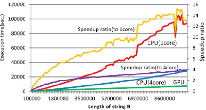
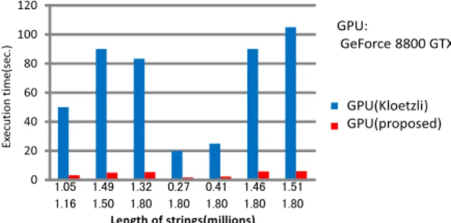
(6) Vol.2014-MPS-97 No.12 2014/3/3. IPSJ SIG Technical Report. A and B measured in millions. The y-axis shows execution times measured in minutes. In Fig. 5, blue bars represent the execution times of Kloetzli et al.’s algorithm on a GPU. Red bars represent the execution times of our proposed algorithm on a GPU. In the shortest case (0.27 million and 1.80 million), the speedup ratio is 12.0. In the longest case (1.51 million and 1.80 million), the speedup ratio is 17.6. The speedup ratio ranges from 10.9 (0.41 million and 1.80 million) to 18.1 (1.49 million and 1.50 million). Fig. 5. A comparison with Kloetzli et al.’s GPU algorithm. rithm on a GPU and our bit-parallel algorithm on a CPU in Fig. 4. We execute the bit-parallel algorithm on a CPU with a single core and four cores. To make a multi-core version of the bit-parallel algorithm, we use task parallelism in OpenMP. In List.2, we execute 15th, 16th, 19th, and 20th lines with task parallelism in OpenMP. In OpenMP 3.0 or later, we can use task parallelism with the notation omp task. Then, the function llcs()s in 15th and 16th lines and lcs()s in 19th and 20th lines are executed respectively in parallel. So, only two cores are used to execute llcs()s in the 1st invocation of lcs(). In the 2nd or later invocation of lcs(), all of four cores are used. In Fig. 4, the green line shows the execution times on a GPU. The red and blue lines respectively show the execution times on a CPU with a single core and four cores. All of the execution times are measured in seconds and shown in the primary y-axis. The orange and purple lines respectively show the speedup ratio of the proposed algorithm on a GPU to the single-core and multi-core version on a CPU. The speedup ratio is shown in the secondary yaxis. In Fig. 4, the length of string A is 20,000,000. The length of string B shown in x-axis increases from 100,000 to 10,000,000. First, we compare the proposed algorithm on a GPU with the single-core version on a CPU. Fig. 4 shows that the proposed algorithm is maximum 15.14 times faster than the single-core version. When the length of B is more than 300,000, the speedup ratio is more than one. Next, we compare the proposed algorithm on a GPU with the multi-core version on a CPU. Fig. 4 shows that the proposed algorithm is maximum 4.09 times faster than the multi-core version . When the length of B is more than 700,000, the speedup ratio is more than one. However, the multi-core version on a CPU is at most 4.03 times faster than the single-core version. The fact implies that the proposed algorithm on a GPU is faster than the single-core version and the multi-core version when lengths of given strings are long enough.. 5. Conclusions In the paper, we have presented a method to implement the bit-parallel LCS algorithm on a GPU and have conducted several experiments on our program based on the method. As a result, the proposed algorithm runs maximum 15.14 times faster than the single-core version of the bit-parallel algorithm on a CPU and maximum 4.09 times faster than the multi-core version of the bitparallel algorithm on a CPU. In addition, the proposed algorithm runs 10.9 to 18.1 times faster than Kloetzli et al.’s algorithm on a GPU. Future works includes optimization to the newest Kepler architecture and measuring execution times on a Kepler GPU. References [1] [2]. [3] [4]. [5] [6] [7] [8] [9] [10] [11]. 4.2 A Comparison with the Existing GPU Algorithm We compared the proposed algorithm on a GPU with Kloetzli et al.’s GPU algorithm. Kloetzli et al. used AMD Athlon 64 CPU and GeForce 8800 GTX GPU. To Compare over the same GPU, we used GeForce 8800 GTX GPU too. In the experiment, we used 2.93 GHz Intel Core i3 530 CPU. The CPU we used in the experiment is faster than Kloetzli et al.’s CPU. So, our environment is not completely equal to Kloetzli et al.’s. However, our algorithm scarcely depends on a CPU. So, we can expect the result does not become quite different. Fig. 5 shows the result. The x-axis shows the length of strings ⓒ 2014 Information Processing Society of Japan. [12]. [13] [14] [15] [16]. R. A. Chowdhury and V. Ramachandran: Cache-oblivious Dynamic Programming, The Annual ACM-SIAM Symposium on Discrete Algorithm (SODA), pp.591–600 (2006) M. Crochemore, C. S. Iliopoulos, Y. J. Pinzon, and J. F. Reid: A Fast and Practical Bit-vector Algorithm for the Longest Common Subsequence Problem, Information Processing Letters, Vol.80, No.6, pp.279–285 (2001) S. Deorowicz: Solving Longest Common Subsequence and Related Problems on Graphical Processing Units, Software: Practice and Experience, Vol. 40, pp.673–700 (2010) A. Dhraief, R. Issaoui, and A. Belghith: Parallel Computing the Longest Common Subsequence (LCS) on GPUs: Efficiency and Language Suitability, The First International Conference on Advanced Communications and Computation (INFOCOMP) (2011) M. Garland and D. B. Kirk: Understanding Throughput-oriented Architectures, Communications of the ACM, Vol.53, No.11, pp.58–66 (2010) D. Gusfield: Algorithms on Strings, Trees and Sequences: Computer Science and Computational Biology, Cambridge University Press (1997) D. S. Hirschberg: A Linear Space Algorithm for Computing Maximal Common Subsequences, Communications of the ACM, Vol.18, No.6, pp.341–343 (1975) D. B. Kirk and W. W. Hwu: Programming Massively Parallel Processors: A Hands-on Approach, Morgan Kaufmann (2010) J. Kloetzli, B. Strege, J. Decker, and M. Olano: Parallel Longest Common Subsequence Using Graphics Hardware, The 8th Eurographics Symposium on Parallel Graphics and Visualization (EGPGV) (2008) E. Lindholm, J. Nickolls, S. Oberman, and J. Montrym: NVIDIA Tesla: A Unified Graphics and Computing Architecture, IEEE Micro, Vol.28, No.2, pp.39–55 (2008) A. Ozsoy, A.Chauhan, and M. Swany: Towards Tera-scale Performance for Longest Common Subsequence Using Graphics Processor, IEEE Supercomputing (SC) (2013) A. Ozsoy, A.Chauhan, and M. Swany: Achieving TeraCUPS on Longest Common Subsequence Problem Using GPGPUs, IEEE International Conference on Parallel and Distributed Systems (ICPADS) (2013) J. Sanders and E. Kandrot: CUDA by Example: An Introduction to General-purpose GPU Programming, Addison-Wesley Professional (2010) J. Sklansky: Conditional-sum Addition Logic, IRE Trans. on Electronic Computers, EC-9, pp.226–231 (1960) M. Vai: VLSI DESIGN, CRC Press (2000) J. Yang, Y. Xu, and Y. Shang: An Efficient Parallel Algorithm for Longest Common Subsequence Problem on GPUs, The World Congress on Engineering (WCE), Vol. I (2010). 6.

(7)