A Method to Maintain the Field Coverage by Static and Mobile Sensor Nodes Using Wireless Charging

全文

(1)Vol.2015-MPS-104 No.4 2015/7/27. IPSJ SIG Technical Report. A Method to Maintain the Field Coverage by Static and Mobile Sensor Nodes Using Wireless Charging Yuki Tsuchiya. Ryo Katsuma. Graduate School of Science Osaka Prefecture University Sakai, Osaka, Japan. Graduate School of Science Osaka Prefecture University Sakai, Osaka, Japan. Abstract—: For wireless sensor networks (WSNs), several studies have addressed the lifetime extension problems using energy harvesting, wireless charging, or mobile sensor nodes. In particular, mobile nodes are effective for adequate field coverage: however, appropriate node movement is critical. We formulate the problem to extend lifetime and maintain field coverage by determining the positions of mobile nodes that can cover the field effectively and charge the batteries of other nodes simultaneously. We propose a coverage algorithm that can cover a field with a minimal number of nodes and a movement algorithm that determines an efficient mobile node movement schedule to charge static nodes. Simulation results, confirm that the energy charging system used by the proposed method can extend WSN lifetime up to 66. I.. I NTRODUCTION. Wireless Sensor Networks (WSNs) are networks constructed with many sensor nodes equipped with wireless communication devices. A major problem with WSNs is the coverage problem. A sensor node can only sense environmental information within a limited circular sensing range. As a result, node deployment must cover the entire field of interest . Node deployment cost can be reduced by placing nodes at appropriate positions. Several studies have attempted to address this issue by adjusting the position of mobile sensor nodes[1][2]. However, efficient movement scheduling of mobile nodes is required because mobile nodes consume significant amounts of energy when moving. An other major problem of WSNs is the lifetime extension problem. A WSN is constructed by many sensor nodes that operate with limited battery power. Conventionally, wired power supplies are employed to recharge batteries. However, wired power systems cannot be used in general WSNs; thus, operating such WSNs for extended periods is challenging. Energy harvesting (EH), which converts natural energy (e.g., light and heat) into electricity, has been considered to address this problem[3][4][5]. In EH, retrieving, recharging, and redeploying sensor nodes are not necessary: thus, it is expected that EH will allow WSNs to operate semi-permanently. However, energy generation by EH is unstable and sometimes insufficient. Thus, wireless charging technology used for cellular phones and a variety of small devices is our focus. It has been reported that electromagnetic induction type wireless charging systems are size and have greater than 80% power efficiency. When mobile nodes have sending devices and static nodes have receiving devices, determining the loci of the mobile ⓒ 2015 Information Processing Society of Japan. nodes when repairing the field coverage and charging batteries of static nodes becomes problematic. We propose a method to allow some mobile nodes with sending devices and solar panels to cover the field, and the other mobile nodes charge the exhausted batteries of the static nodes. The proposed algorithm is comprised of a coverage algorithm and a movement algorithm. When a field is covered by static as well as mobile sensor nodes, the coverage algorithm determines the positions of a minimal number of mobile nodes that can cover the field by determining enclosed regions that are not covered by sensor nodes. The movement algorithm determines the destination points of free mobile nodes. Our simulation results show that the proposed method extends WSN lifetime up to 66% for a 100 × 100 [m2 ] field with 20 - 115 nodes. We have confirmed that the coverage algorithm can repair field coverage with a sufficiently small number of nodes. We have also confirmed that employing the proposed method in a honeycomb structure is more effective than random deployment. II.. A SSUMPTIONS AND P ROBLEM AND FORMULATION. A. Target WSNs We target WSNs constructed with a single sink node and static and mobile sensor nodes. Here, a sink node is denoted B. Static and mobile sensor nodes have batteries and devices for sensing and radio communication. The capacity of the battery is denoted E. The residual battery power of node s at time t is denoted s.energy(t). The sensing range and communication range are denoted Rs and Rc , respectively. Both types of sensor nodes sense environmental data every duty cycle I (a sink collects the environmental information from all sensor nodes every I minutes). We assume that a mobile sensor node can move to specified destination, charge its battery using an equipped solar panel and send electric energy to a static sensor node using the equipped wireless charging system’s sending device. The speed of a mobile node is constant value v. Note that a static sensor node can charge using only its wireless charging receiving device. If the distance between the sending and receiving devices is less than dc , a static node can charge its battery from a mobile node. Here, a field with height Fheight and width Fwidth is given, in which Nstatic static sensor nodes are initially deployed. Then, Nmobile mobile sensor nodes are deployed to cover the field completely and charge the batteries of the static nodes. The position of sensor node s at time t is denoted s.pos(t). The destination point of 1.

(2) Vol.2015-MPS-104 No.4 2015/7/27. IPSJ SIG Technical Report. mobile node p at time t is denoted s.dest(t). A sensor node can know its own position and the positions of other nodes using GPS and wireless communication.. coefficient. c([t, t+u]) is expressed by Formula (8). icnight + jccloudy + kcsunny c([t, t + u]) = i+j+k. B. Definitions. Here, i, j, and k are the rates of night, cloudy, and sunny periods during [t, t + u], respectively.. A sensor node has finite battery power, and it is not feasible to replace batteries physically when they are exhausted. Battery power is consumed by sensing, moving, wireless communication, and supplying electric power. On the other hand, battery power can be charged by solar power generation and the electric power supplied by a mobile node. The power for consumed sensing x[bit] data Sens(x) is expressed by Formula(1). Sens(x) = Eelec x + Esens. (1). Here, Esens and Eelec are constant values that represent the power required for sensing and information processing, respectively.. (8). C. Problem formulation The inputs to the target problem are target field (Fwidth × Fheight ), the positions of the sink node and static nodes, the initial battery power of each sensor node, sensing range, and constants Esens , Eelec , ϵamp , ϵwc , and ϵsolar . The outputs are the position of each mobile node for each time t and the node pairs for battery power supply at each time t. We refer to these node positions as the node schedule. Note that the field must always be covered by sensor nodes. This condition is expressed by Formula (9). ∀pos ∈ F ield, ∀t ∈ T ime, cover(pos, t) ≥ 1 (9). Consumed powers T rans(x, d) and Recep(x) required to transmit x[bit] for d[m] and receive x[bit] are expressed by Formulas (2) and (3), respectively [6].. Here, Cover(pos, t) is the number of nodes covering the point pos at time t. T ime and F ield represent set of the WSN termination time and set of the field, respectively.. T rans(x, d) = Eelec × x + εamp × x × d2. (2). Recep(x) = Eelec × x. (3). If node s with position s.pos(t) at time t moves to s’s destination point s.dest(t), the residual battery power of s should be greater than the energy consumed by moving. This constraint is expressed by Formula (10).. Here, ϵamp is a constant value that represents the power required for signal amplification. Consumed power M ove(d) required to move d [m] is expressed by Formula (4) [5]. M ove(d) = Emove d. (4). Here, Emove is a constant value that represents the power required to move a node 1 [m]. Using the wireless charging system, mobile sensor node p consumes its energy to charge the battery of static node q. Consumed power Csend (y) required to send the electric power for y [sec] is expressed by Formula (5). Csend (y) = ϵwc y (5) Here, ϵwc is a constant value that represents the energy consumption of the wireless charging system. The energy of charged by the wireless charging system Crecep (y)for y [sec] is expressed by Formula (6). Crecep (y) = θϵwc y (6) Here, θ represents the charging efficiency (0 ≤ θ ≤ 1). If θ = 1, the energy consumption of a mobile node equals the charged energy of a static node. A mobile node can charge its battery by solar power generation. The amount of generated solar power depends on the intensity of solar radiation, which varies according to changing environmental conditions. We denote the intensity of solar radiation at night, during a cloudy day, and during a sunny day as cnight , ccloudy , and csunny , respectively. The amount of solar power generated at an average solar radiation intensity c([t, t + u]) from time t to t + u is expressed by Formula 7 [4]. Csolar (c([t, t + u])) = ϵsolar uc([t, t + u]) (7) Here, ϵsolar is the charged energy amount per unit time ⓒ 2015 Information Processing Society of Japan. ∀t ∈ T ime, s.energy(t) − M ove(|s.dest(t) − s.pos(t)|) + |s.dest(t) − s.pos(t)| Csolar (c([t, t + ])) > 0 (10) v Here,|s.dest(t) − s.pos(t)| represent the moving distance. If mobile node p charges the battery power of static node q at time t for ut seconds, the residual battery power of p should be greater than the energy consumed for charging. ∀t ∈ T ime, s.energy(t)−Csend (ut )+Csolar (c([t, t+ut ]) > 0 (11) Our purpose is to determine a node schedule that maximizes WSN operation time T . The objective function is shown in Formula (12). maximize(T ) (12). III.. P ROPOSED METHOD. A. Coverage algorithm First, the polygon-finding algorithm included in the coverage algorithm finds all areas that are not covered by static nodes. Next, the coverage algorithm determines efficient positions for the mobile nodes that will cover the uncovered areas. Finally, the mobile nodes are deployed to each position. To find each uncovered polygon that inscribes an uncovered area, the polygon-finding algorithm finds all uncovered intersections. An uncovered intersection is an intersection that is not covered by sensor nodes and is made up of two elements, i.e., edges of the target field and sensing range circles of the sensor nodes. Note that an uncovered polygon, whose vertices are uncovered intersections, exists if and only if an uncovered area exists. 2.

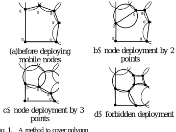
(3) Vol.2015-MPS-104 No.4 2015/7/27. IPSJ SIG Technical Report. q1. q2. q3. q2. q3. q4. q4 q1. q6. q6. q5. (a)before deploying mobile nodes. q1. q5. （b）node deployment by 2 points. q2 q3. q5. q4. （c）node deployment by 3 （d）forbidden deployment points Fig. 1.. and becomes a coverage mode node. Note that free mode nodes do not perform sensing.. A method to cover polygon Q. The coverage algorithm minimizes uncovered polygons by placing nodes at appropriate positions in the polygons sequentially until the polygons no longer exist. Here, we denote a set of uncovered polygon vertices found by the polygon-finding algorithm as Q = {q0 , q1 , q2 , · · ·} , which qi and qi+1 are adjoined vertices. Two sensor nodes a and b that construct vertex qi is denoted by qi .s1 and qi .s2 , respectively. Note that qi .s2 and qi+1 .s1 represent the same sensor node b. Similarly, qi−1 .s2 and qi .s1 represent the same sensor node a. If the distance between qi and qi+2 is within diameter 2Rs of the sensing range circle, the candidate position of a node that covers qi , qi+1 , and qi+2 exists. This position is the circumcenter of the triangle whose vertices are qi , qi+1 , and qi+2 . If no such node position includes these three vertices, the candidate position is the center of the circle that inscribes qi and qi+1 . The coverage algorithm places the mobile node at one of these candidate positions such that the area that is newly covered by the mobile node is maximized. Here, if the mobile node placed at the candidate position divides the uncovered polygon into two or more polygons, such a position is eliminated as a candidate. In order to simplify the problem, our algorithm makes the outer side destination have priority. For example, uncovered polygon Q is constructed by uncovered intersections q1 , q2 , q3 , q4 , q5 , and q6 as shown in Fig. 1 (a). The mobile node is placed at the center of the circle that inscribes q1 and q2 , because the area whose size is newly covered by the mobile node is maximized as shown in Fig. 1 (b). Then, the distance between q2 and q4 in Fig. 1 (b) is less than 2Rs , and the mobile node is placed at the circumcenter of the triangle whose vertices are q2 , q3 , and q4 (Fig. 1 (c)). On the other hand, the mobile node is not placed at a position such that the uncovered polygon becomes divided as shown in Fig. 1 (d). B. Movement algorithm The movement algorithm allows field coverage to be maintained for long periods. We set two modes for each mobile node, i.e., a coverage mode and a free mode. A coverage mode mobile node moves to the candidate position calculated by the coverage algorithm. Note the number of coverage mode nodes is fixed. The other nodes operate in free mode. If the residual battery power of a coverage mode node becomes low, the free mode node moves to the position of the coverage mode node ⓒ 2015 Information Processing Society of Japan. In the movement algorithm, nodes communicate residual battery power and power-generation efficiency information to each other, and the sink node forecasts node s whose residual battery power will be depleted rapidly. If s is a free mode node, s charges its battery by solar power at its current position. If s is a static node or a coverage mode node, it seeks another mobile node n1 with sufficient battery power. If mobile node n1 is a free mode node, then it moves to the position of node s and performs wireless charging or changes n1 ’s mode to coverage and s’s mode to free: otherwise, s seeks the nearest c c free mode node n2 . En1 and En2 are the estimated residual battery power of nn1 and nn2 when n2 move to the position of n1 and nn1 moves to the position of s (this type of movement d d is referred to as cascade movement [2]. En1 and En2 are the estimated residual battery power of nn1 and nn2 when n2 moves directly to the position of s. The movement algorithm compares the minimum values of the estimated residual battery c c power En1 and En2 to E1d and E2d by these two movement types and selects the movement type with greater estimated residual battery power. The movement algorithm runs when a node whose residual battery power is less than Ll exists. Here, the average residual battery power among all nodes is denoted L. 1) Movement algorithm: 1). 2). 3). 4) 5). If node s whose residual battery power is a less than L l is free mode node, then s’s battery is charged by solar energy generation and the algorithm terminates, else seek the nearest mobile node n1 whose battery power is greater than L. If n1 is a free mode node, then move n1 to the position of s and proceed to Step 5, else seek mobile node n2 that has more than L battery power and is the nearest node from s. d d by and En2 Estimate the residual battery power En1 moving n2 to the position of s directly, and estimate E1c and E2c by moving n2 to n1 ’s position and n1 to the position of s (cascade movement). Select the movement of the greater minimum value of E1c and E2c , or E1d and E2d . Mobile nodes are then moved. If node s is a static node, the moved mobile node performs wireless charging, else s and the moved mobile node exchange modes. IV.. P ERFORMANCE EVALUATION. To evaluate the effects of the proposed features, we compared the proposed method with a method whose battery charging mechanism has not been validated (hereafter, simple method ). The common parameter settings in our simulations are shown in Table. I. The network topology is a mesh rooted at the sink node. Each sensor node sends data to the upper node that has maximum residual battery power. A. Coverage algorithm evaluation In this simulation, n static nodes were deployed initially, and the number of mobile sensor nodes required for complete 3.

(4) Vol.2015-MPS-104 No.4 2015/7/27. IPSJ SIG Technical Report TABLE I.. C OMMON PARAMETER. SETTINGS IN THE SIMULATIONS. Size of target field Sensing radius Rs Duty cycle I Data size Battery capacity E Power consumption coefficient for data processing Eelec Power consumption coefficient for signal amplification ϵamp Power consumption coefficient for sensing Esens Power consumption for moving Efficiency of wireless charging θ. 100 × 100 [m2 ] 20 [m] 15 [min] 256 [bit] 8640 [J] 50 [nJ/bit] 100 [pJ/bit/m2 ] 0.018 [J/bit] 1680 [mW] 0.8. Fig. 2. The number of nodes Fig. 3. WSN lifetime with 15 static needed by the coverage algorithm nodes. field coverage was measured. The average results of 10 trials are shown in Figure. 2. The coverage algorithm required 18 sensor nodes (five randomly deployed static nodes and 13 mobile nodes) to cover the 100 × 100 [m2 ] field. Note that a honeycomb structure required 14 nodes to cover the same field. The coverage algorithm can cover the field with a small number of nodes. B. Evaluation of the proposed method In this simulation, we measured the lifetime of the WSN lby changing the number of mobile sensor nodes. WSN operation was terminated when battery power of at least one node was depleted. 1) Changing the number of mobile nodes: Figure. 3 shows the WSN lifetime with 15 static nodes and various numbers of mobile nodes. We confirmed that WSN lifetime is extended by increasing the number of mobile nodes. We confirmed that the proposed method achieves 66% longer WSN lifetime than the simple method with 100 mobile nodes. However, the difference between the proposed method and the simple method with 20 mobile nodes was not significant because the total energy generation of 100 mobile nodes is grater than 20 mobile nodes. WSN lifetime is extended with increased total energy generation.. of a hexagon inscribed in a circle whose radius is Rs .The honeycomb structure is the most efficient deployment [1]. The honeycomb structure requires 14 static nodes to cover a 100 × 100 [m2 ] field, as described in Subsection IV-A. We added mobile sensor nodes to WSNs constructed with only static sensor nodes that have already consumed one-half and onequarter if their battery power on average. The durations from initial deployment of the static nodes until one-half and onequarter battery power was consumed was 189.4 [h] and 298.7 [h], respectively. Here, we describe these two cases (i.e., onehalf and one-quarter battery consumption). For each case, we measured the lifetime extension achieved by adding mobile nodes. Figures 4 and 5 show the one-half and one-quarter cases, respectively. As can be seen in both figures, the proposed method extends WSN lifetime linearly relative to the number of mobile nodes. However, the degree of lifetime extension is gradual around 550–600 [h]. With 30 mobile nodes, Figs. 3 and 4 show 793.2 [h] and 591.5 [h] lifetime extensions. In the one-half case, the WSN lifetime is 591.5 + 189.4 = 780.9. Although no mobile node was used for 189.4 [h], the lifetime of the one-half case was similar to the randomly deployed case. Thus, we confirmed that the proposed method with a honeycomb structure can extend WSN lifetime. V.. We have proposed a method to extend WSN lifetime using two energy charging systems. The proposed algorithm includes a coverage algorithm and movement algorithm. The coverage algorithm determines the positions of mobile nodes that cover areas not covered by static nodes. The movement algorithm determines the destination of nodes whose batteries need to be charged by mobile nodes. Our simulation results, confirm that the proposed method with a honeycomb structure deployment can extend WSN lifetime. In future, we plan to decentralize the proposed algorithm for scalability. R EFERENCES [1]. [2]. [3]. [4]. [5]. Fig. 4. case). Honeycomb structure (1/2 Fig. 5. case). Honeycomb structure (1/4. 2) Honeycomb structure deployment: In this simulation, each static sensor node was deployed as the center point ⓒ 2015 Information Processing Society of Japan. C ONCLUSION. [6]. Xiaole Bai, Ziqiu Yun, Dong Xuan, Biao Chen and Wei Zhao: “Optimal Multiple-Coverage of Sensor Networks,” Proc. of IEEE Int’l. Conf. on INFOCOM, pp. 2498–2506, 2011. You-Chiun Wang, Fang-Jing Wu and Yu-Chee Tseng: “Mobility management algorithms and applications for mobile sensor networks,” J. of Wireless Communications and Mobile Computing, Vol. 12, Issue 1, pp.7–21, 2012. Davide Brunelli, Luca Benini, Clemens Moster, and Lothar Thiele, : “An Efficient Solar Energy Harvester for Wireless Sensor Nodes,” Proceedings of the conference on Design, automation and test in Europe pp 104-109 (2008) Masaru Eto, Ryo Katsuma, Morihiko Tamai, and Keiichi Yasumoto: “Efficient Coverage of Agricultural Field with Mobile Sensors by Predicting Solar Power Generation,” Proc. of IEEE Int’l. Conf. on The 29th IEEE International Conference on Advanced Information Networking and Applications (AINA), pp. 62–69, 2015. Rahimi, M., Shah, H., Sukhatme, G.S., Heideman, J., Estrin, D. “Studying the Feasibility of Energy Harvesting in a Mobile Sensor Network,” Proc. of the IEEE Int’l. Conf. on Robotics and Automation (ICRA), pp.19–24, 2003. Heinzelman, W.R., Chandrakasan, A., Balakrishnan, H. “Energyefficient communication protocol for wireless microsensor networks,” Proc. of the 33rd Hawaii Int’l. Conf. on System Sciences (HICSS 2000) , pp.1–10, 2000.. 4.

(5)