Rapid Feature Selection Based on Random Forests for High-Dimensional Data

全文

(1)IPSJ SIG Technical Report. Vol.2012-MPS-89 No.3 2012/7/16. Rapid Feature Selection Based on Random Forests for High-Dimensional Data Hideko KAWAKUBO, Hiroaki YOSHIDA Graduate School of Humanities and Sciences, Ochanomizu University, Tokyo, Japan. Abstract— One of the important issues of machine learning is obtaining essential information from high-dimensional data for discrimination. Dimensionality reduction is a means to reduce the burden of dimensionality due to large-scale data. Feature selection determines significant variables and contributes to dimensionality reduction. In recent years, the random forests method has been the focus of research because it can perform appropriate variable selection even with high-dimensional data holding high correlations between dimensionality. There exist many feature selection methods based on random forests. These methods can appropriately extract the minimum subset of important variables. However, these methods need more computation time than the original random forests method. An advantage of the random forests method is its speed. Therefore, this paper aims to propose a rapid feature selection method for highdimensional data. Rather than searching the minimum subset of important variables, our method aims to select meaningful variables quickly under the assumption that the number of variables to be selected is determined beforehand. Two main points are introduced to enable faster calculations. One is reduction in the calculation time of weak learners. The other is adopting two types of feature selection: “filter” and “wrapper.” In addition, although most present methods use only “mean decrease accuracy,” we calculate the magnitude of features by combining “mean decrease accuracy” and “Gini importance.” As a result, our method can reduce computation time in cases where generated trees have many nodes. More specifically, our method can reduce the number of important variables to 0.8% on an average without losing the information for classification. In conclusion, our proposed method based on random forests is found to be effective for achieving rapid feature selection. Keywords: feature selection; variable selection; random forests; Gini importance;. 1. Introduction In recent years, feature selection for dimensionality reduction is becoming increasingly important in machine learning. Feature or variable selection enables improving accuracy by excluding redundant variables and facilitates the interpretation of complex data structures as well as reduces calculation time for predictors. Therefore, variable selection for high-dimensional data plays an important role in many ⓒ 2012 Information Processing Society of Japan. areas including text processing of internet documents, gene expression array analysis and combinatorial chemistry. In this paper, we propose a rapid feature selection method for high-dimensional data. There are three types of variable selection: “filter,” “wrapper,” and “embedded” [1], [2]. “Filter” selects subsets of variables in a preprocessing step, independent of the chosen predictor. “Wrapper” utilizes the learning machine of interest as a black box to score subsets of variables according to their predictive power. “Embedded” performs variable selection during the training process and is usually specific to given learning machines. The random forests (RF) method [3] based on the wrapper method has been widely recognized as a practical method of variable selection. In recent years, the RF method has also been applied to feature selection for hyperspectral imagery and gene selection of microarray data [4], [5]. Furthermore, the demand for variable selection has been increasing. The RF method has two types of variable importance measures. One involves the evaluation of “out-of-bag (OOB) errors” introduced to estimate prediction errors. Several feature selection methods using this measure have been proposed [6], [7], [8]. The other measure is derived from the Gini index and is called “Gini importance.” This measure is biased toward predictor variables with many categories [9]. However, it is particularly effective with data that have a high dimensionality and small sample size [10]. There also exists a feature selection method using “Gini importance” [11]. These feature selection methods, which are extended RF methods, can appropriately extract the minimum subset of important variables. Because the RF method itself is stochastic, the subsets obtained by these methods are only a candidate of the optimal solution; moreover, if sufficient computation time is provided, these methods are attractive. In this paper, we assume that the number of important variables to be selected is decided beforehand and propose a fast method to select meaningful variables with a high accuracy. As a result of investigating the ranking of important variables derived from various datasets by using the original RF method, we obtain the following empirical rule: the rankings drawn from two types of variable importance measures slightly differ, whereas the members of the top ranked variables are almost the same. Based on this empirical rule, we improve the original RF method and successfully reduce 1.

(2) Vol.2012-MPS-89 No.3 2012/7/16. IPSJ SIG Technical Report. computation time, especially in cases where generated trees have many nodes. In addition, in our method, the number of important variables is reduced to 0.8% on an average without losing the information for discrimination. In conclusion, our proposed method based on RF is effective to achieve rapid variable selection. The reason why our method is successful is not solved mathematically; the results obtained by our method are very interesting. In the following section, we review RF and “Gini importance”; we explain our proposed method in section 2.. 1.1 Random forests algorithm The RF method creates multiple trees using classification and regression trees (CART) [12]. When constructing a tree, the RF method searches for only a random subset of input variables at each splitting node and the tree grows fully without pruning. The RF method is recognized as a specific instance of bagging. Random selection of variables at each node decreases the correlation among trees in a forest, thus forest error rate decreases. The random subspace selection method has been demonstrated to perform better than bagging when there are many redundant variables contributing to discrimination among classes [13], [14], [15]. The computational load of the RF method is comparatively√ light. The computation time is on the order of ntree mtry n log n, where ntree is the number of trees, mtry is the number of variables used in each split, and n is the number of training samples [3], [4]. In addition, when a separate test set is not available, an OOB method can be used. For each newly generated training set, one-third of the samples are randomly excluded; these are called OOB samples. The remaining (in-thebag) samples are used for building the tree. For accuracy estimation, votes for each sample are counted every time a sample is included among OOB samples. A majority vote determines the final label. The OOB error estimates are unbiased in many tests [3]. The number of mtry is defined by a user, and it is insensitive to the algorithm. The RF algorithm (for both classification and regression) is as follows: 1) Draw ntree bootstrap samples from the original data. 2) For each bootstrap sample, randomly sample mtry predictors (variables) at each node, grow an unpruned classification or regression tree, and choose the best split among these variables (rather than choosing the best split among all variables). 3) Predict new data by aggregating the predictions of ntree trees (i.e., majority vote is used for classification, average is used for regression). Based on training data, an error rate estimate can be obtained as follows: 1) At each bootstrap iteration, predict test data not in the bootstrap sample (what Breiman calls “out-of-bag” ⓒ 2012 Information Processing Society of Japan. or OOB data) using a tree grown with the bootstrap sample. 2) Aggregate the OOB predictions. Calculate their error rate, and call it OOB error rate estimate. The RF method performs efficiently for large datasets and can handle thousands of input variables. The RF algorithm has been demonstrated to have excellent performance in comparison to other machine learning algorithms [3], [16], [17].. 1.2 Gini importance The RF method has extremely useful byproducts, for instance, variable importance measures [3], [18]. There are two different algorithms for calculating variable importance. The first algorithm is based on the Gini criterion used to create a classification tree, CART [12]. In this paper, we call the measure “Gini importance.” At each node, decreases in Gini impurity are recorded for all variables used to form the split. Gini impurity ∆GI(t) is defined as follows: ∆GI(t) = Pt GI(t) − PL GI(tL ) − PR GI(tR ). Here, GI(t) is called the Gini index and is defined as follows: ∑ p(k | t)2 , GI(t) = 1 − k. where p(k | t) is the rate at which class k is discriminated correctly at node t, GI(tL ) is a Gini index on the left side of the node, GI(tR ) is a Gini index on the right side of the node, Pt is the number of samples before the split, PL is the number of samples on the left side after the split, and PR is the number of samples on the right side after the split. The Gini criterion is used to select the split with the highest impurity at each node. The average of all decreases in Gini impurity yields the “Gini importance” measure. The second algorithm is based on OOB observations. In this paper, we call the measure “mean decrease accuracy.” Although the structure of a decision tree provides information concerning important variables, such an interpretation is difficult for hundreds of trees in an ensemble. One additional feature of RF is the ability to evaluate the importance of each input variable by the OOB estimates. To evaluate the importance of each variable, the values of each variable in the OOB samples are allowed to permute. The perturbed OOB samples will run down each tree again. Then, the difference between the accuracies of the original and perturbed OOB samples over all trees in RF are averaged. Variable importance of “mean decrease accuracy” is defined as follows: Let Xj (j = 1, · · · , M ) be the permuted variables, where M is the number of all variables. Xj and the remaining nonpermuted predictor variables together form a perturbed OOB sample. When Xj is used to predict the response for the OOB sample, the prediction accuracy (i.e., the number of samples classified correctly) decreases 2.

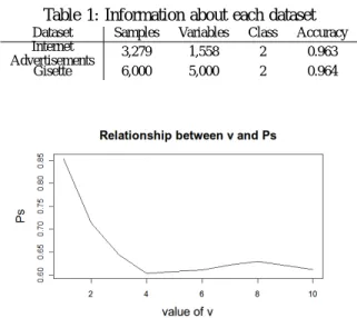
(3) Vol.2012-MPS-89 No.3 2012/7/16. IPSJ SIG Technical Report. substantially, if the original variable Xj is associated with the response. For each tree f of the forest, consider the associated OOBf sample (data not included in the bootstrap samples used to construct f ). The error of a single tree f in this OOBf sample is denoted by errOOBf . Now, randomly permute the values of Xj in OOBf to get a permuted sample denoted by OOBf j and compute errOOBf j , the error of predictor f in the perturbed sample. Variable importance of Xj is then equal to V I(Xj ) =. Table 1: Information about each dataset Dataset Internet Advertisements Gisette. Samples 3,279 6,000. Variables 1,558 5,000. Class 2 2. Accuracy 0.963 0.964. 1 ∑ (errOOBf − errOOBfj ), ntree f. where the summation is over all trees f of RF and ntree denotes the number of trees of RF.. 2. Rapid Feature Selection Based on Random Forests We investigate the ranking of important variables derived from various datasets by using the original RF method and obtain an empirical rule: the rankings of important variables obtained from “Gini importance” and “mean decrease accuracy” differ slightly, whereas the members of the top ranked variables are almost the same. Thus, if we can determine these members of the top ranked variables obtained from “Gini importance,” we can rank variable importance by “mean decrease accuracy.” To realize this idea, we combine “Gini importance” and “mean decrease accuracy” as “filter” and “wrapper.” We propose an improved method of RF and call it “rapid feature selection” method (RFS). After reducing meaningless variables by “filter,” rapid feature selection evaluates variable importance by “wrapper.” “Gini importance” can be acquired from the generation process of weak learners, thus it is convenient to use the “Gini importance” measure as a “filter.” However, sometimes we cannot obtain high accuracy by only using such a “filter.” On the other hand, “mean decrease accuracy” is high; “mean decrease accuracy” is computationally heavy because it has to call on the learning algorithm to evaluate each subset. The rapid feature selection algorithm is as follows: 1) Exclude OOB data and draw ntree bootstrap samples from training data. 2) For each bootstrap sample, randomly sample mtry variables, grow a tree up to the first node, and record all Gini impurities generated in the calculation process. 3) Choose the top v variables that are candidates for the best split, give a score that reflects the top ranked v variables for ntree trees, and aggregate all scores. 4) To select the top s important variables, choose the top se variables at this point (se is larger than s). 5) Rank se variables by “mean decrease accuracy” of the original RF method and select the top v variables. ⓒ 2012 Information Processing Society of Japan. Fig. 1: Simulation: Relationship between v and Ps . Number of variables: 1, 558.. In the case that some variables are correlated, CART can choose the best split. However, CART needs the calculation of Gini impurity up to 2n−1 − 1 times in the worst case, where n is the number of samples in each bootstrap sample. Thus, reducing the calculation time of CART is a significant issue in this method. To reduce the calculation time of CART, some RF applications have an option to stop calculation at the first node. This option is effective in reducing computation time; however, the appropriate evaluation of important variables cannot be obtained. Necessary information will be insufficient when v = 1 owing to the nature of the data; therefore, we set a parameter v. Under the assumption that CART can accurately rank variables and all variables are independent, we simulated the behavior of these parameters. In the simulation, we used the number of variables from Table 1. Let Ps be a probability that the top s variables are included in the top se variables. The relationship among Ps and the other parameters are shown in Figures 1,2,3,4 and 5. The parameters that are not a target of the investigation are set as follows: se = 35, s = 20, v = 5 and ntree = 100 for the case of 1, 558 variables (Figures 1,3,4 and 5), and se = 70, s = 55 and ntree = 100 for the case of 5, 000 variables (Figure 2). From Figures 1 and 2, we can find that the optimal v changes owing to the number of variables. Because CART cannot necessarily rank variables correctly and all variables are not independent in real data, in practice, the optimal v differs from the result of the simulation. Without changing the parameter setting, we conducted a experiment using real data to investigate about v. Internet advertisement dataset in Table 1 was chosen as a real data with 1, 558 variables. This 3.

(4) Vol.2012-MPS-89 No.3 2012/7/16. IPSJ SIG Technical Report. Fig. 2: Simulation: Relationship between v and Ps . Number of variables: 5, 000.. Fig. 4: Simulation: Relationship between ntree and Ps . Number of variables: 1, 558.. Fig. 3: Simulation: Relationship among v, se and Ps . Number of variables: 1, 558.. Fig. 5: Simulation: Relationship between se and Ps . Number of variables: 1, 558.. experiment was conducted using rapid feature selection. Figure 6 shows that the accuracy of this real data is insensitive to the value of v. It is difficult to predict the optimal v. However, under the condition that v is 5 or more, we found that the behavior of Ps is stabilized if se changes. Figure 3 supports this empirical rule. Thus, we conducted experiments by provisionally setting v = 5, as described in the following chapter. Prediction of v is one of the future work. Figure 4 expresses the relationship between ntree and Ps , and Figure 5 the relationship between se and Ps . These Figures show a following relationship: The more the value of ntree or se becomes large, the more the value of Ps approaches 1. Under the assumption that s is determined beforehand, we consider that all parameters should be set to satisfy the following condition: mtry ×. s × Ps (s, se ) × ntree ≥ s. M. It is expected that the maximization of Ps and minimization of se and ntree are realized simultaneously. When 1.5s = se , mtry × ntree/M = 2.5, Ps is about 0.5 is considered as one index. ⓒ 2012 Information Processing Society of Japan. 3. Experiment First, we conducted experiments to verify the performance of rapid feature selection compared with another well-known method. For comparison, we chose principal component analysis (PCA). PCA provides factor loading amount and accumulated contribution rate for variable selection. By using these values, we selected meaningful variables. Next, to determine whether “mean decrease accuracy” used as “wrapper” in our method works effectively, we compared the performance of rapid feature selection and a method that employs only “filter” in rapid feature selection. In this paper, we refer to this method as “first split” (FS). First split does not use the evaluation from mean decrease accuracy. The first split algorithm is simple and its steps 1) to 3) are the same as those of the rapid feature selection algorithm, except that there is no need to exclude OOB data. Because “mean decrease accuracy” consumes computation time, an alternative method is desired. To this end, we introduce weighted sampling. Gender et al. suggested selecting random mtry inputs according to a distribution derived from the preliminary ranking given by a pilot estimator [19]. Based on their concept, we propose another method for rapid variable selection. In this paper, we call this method “first 4.

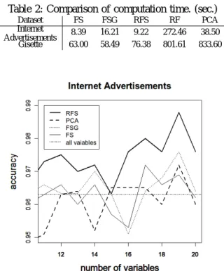
(5) Vol.2012-MPS-89 No.3 2012/7/16. IPSJ SIG Technical Report. Table 2: Comparison of computation time. (sec.) Dataset Internet Advertisements Gisette. FS 8.39 63.00. FSG 16.21 58.49. RFS 9.22 76.38. RF 272.46 801.61. PCA 38.50 833.60. Fig. 6: Experiment: Relationship between v and accuracy. Dataset: Internet Advertisements.. split Gibbs” (FSG). After performing the first split algorithm, first split Gibbs normalizes the score derived from step 3) of the first split algorithm. Then, let the normalized values be Gi (i = 1, · · · , M ) and calculate the Gibbs distribution by substituting Gi as a potential. The probability function of the Gibbs distribution is defined as follows: exp(−βGi ) Pi = ∑M i=1 exp(−βGi ). (β > 0).. To sample mtry variables according to the Gibbs distribution, first split Gibbs repeats the first split algorithm once again. Weighted samplings are performed by adjusting the parameter β. The original RF method samples mtry variables according to the uniform distribution. Substituting β = 0 for the probability function of the Gibbs distribution, the resulting distribution equals the uniform distribution. When we substitute large values for β, the probability that the variables with large Gi are chosen increases. Using high-dimensional data from UCI Machine Learning Repository, we investigate computation time and quality of variable selection, that is, whether important variables are properly selected. After performing PCA and the three methods, the accuracy of each is compared using only the variables selected. The score at step 3) of the rapid feature selection algorithm is obtained by giving the 1/r points to the rth variable (r = 1, · · · , v). As datasets for the experiment, we use an internet advertisements dataset and the Gisette dataset. Readers can refer to the details of these datasets at (http://archive.ics.uci.edu/ ml/data-sets/Internet+Advertisements, http://archive.ics.uci. edu/ml/datasets/Gisette). The experiment using internet advertisements results in trees with several nodes. On the other hand, the experiment using the Gisette dataset results in trees with many nodes. For each dataset, Table 1 shows the number of samples and variables and the accuracy calculated using all variables. The computation environment is as follows: CPU Phenom X4 9950, OS Windows7 Professional 64bit, RAM 8GB. ⓒ 2012 Information Processing Society of Japan. Fig. 7: Comparison of accuracy calculated using selected variables only. Method: RFS, PCA, FS and FSG. Dataset: Internet Advertisements.. 4. Results and discussion Table 2 shows the computation time of each method. The parameters used in this experiment are set as follows: √ mtry = ⌊ M +0.5⌋, ntree = 200, v = 5, se = 20, s = 15. First split Gibbs and rapid feature selection need two-stage estimations. At each stage, ntree = 100 is set. Computation time depends on the property of a dataset, thus the ranking of first split, first split Gibbs, and rapid feature selection varied slightly. However, the computation time of the rapid feature selection method was always lower than the original RF. From this result, rapid feature selection was found to be a much faster method than the original RF method. The results of the accuracy calculated using selected variables only are plotted in Figures 7, 8 and 9. We can compare rapid feature selection, PCA, first split and first split Gibbs from these figures. In this experiment, the accuracy in Table 1 is used as the evaluation criterion regarding whether the information for classification is maintained. The result showed that rapid feature selection can maintain accuracy even if the number of dimensions becomes high. The parameters used in this experiment are set as follows: √ mtry = ⌊ M + 0.5⌋, ntree = 200, v = 5, β = 100 ,s = 10 − 20, se = 25 √ − 35 for the internet advertisements dataset and mtry = ⌊ M + 0.5⌋, ntree = 200, v = 5, β = 100 ,s = 45 − 55, se = 60 − 70 for the Gisette dataset. 5.

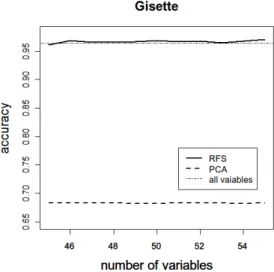
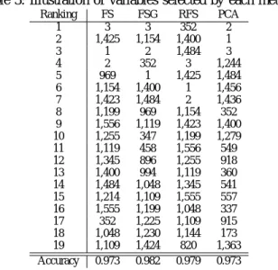
(6) Vol.2012-MPS-89 No.3 2012/7/16. IPSJ SIG Technical Report. Fig. 8: Comparison of accuracy calculated using selected variables only. Method: RFS and PCA. Dataset: Gisette.. Fig. 9: Comparison of accuracy calculated using selected variables only. Method: RFS, FS and FSG. Dataset: Gisette.. Rapid feature selection needs two-stage estimations. At each stage, ntree = 100 is set. From the results, we found that rapid feature selection can select important variables more accurately than first split and first split Gibbs. In addition, we found that trees with many nodes do not affect the results. Even if we reduced the number of variables to 0.6% for the internet advertisements dataset and 0.92% for the Gisette dataset, the accuracy did not fall below the evaluation criterion. These results indicate that rapid feature selection maintains the information for discrimination after variable selection. The ranking of variables selected by each method are illustrated in Table 3. The results of the internet advertisements ⓒ 2012 Information Processing Society of Japan. dataset are used for this experiment. The parameters √ used in this experiment are set as follows: mtry = ⌊ M + 0.5⌋, ntree = 200, v = 5, β = 100, se = 34, s = 19. In the table, the values under the three methods represent the ID number of the variables. In this case, the ID number is up to 1, 558. Both rapid feature selection and first split select almost the same variables because rapid feature selection is based on first split. Here, about 11% of the variables are replaced, and the accuracy increased as a result of this change. Because “mean decrease accuracy” is introduced in step 5) of the rapid feature selection algorithm, the accuracy of rapid feature selection is higher than that of first split. Therefore, the effectiveness of the “wrapper” method was verified through this experiment. First split Gibbs is also based on first split and about 37% of variables are replaced by weighted samplings. In this case, the estimation by sampling mtry variables according to the Gibbs distribution was successful and accuracy was improved. However, owing to the nature of the data, first split itself can correctly select important variables. In contrast, first split Gibbs reduces accuracy rate in such a situation. This phenomenon can be observed in Figure 9. Adjusting the value of β is difficult, thus first split Gibbs has a problem of time to adjust the value of β. However, first split Gibbs is a promising method as an alternative method of “mean decrease accuracy,” if adjustment of β can be performed well. Our study showed that rapid feature selection performs faster than the original RF method and can correctly select important variables even if trees with many nodes are generated. Rapid feature selection cannot search the minimum subset of significant variables for discrimination. However, under the conditions that the number of variables to be selected is predefined, rapid feature selection is useful to rapidly search essential variables.. 5. Conclusion In this paper, we proposed the rapid feature selection method based on an empirical rule: the rankings of important variables obtained from “Gini importance” and “mean decrease accuracy” differ slightly, whereas the members of the top ranked variables in RF are almost the same. If this empirical rule is solved mathematically, the reason our method is successful becomes clear. The rapid feature selection method involves a two-step estimation. As the first step, candidates for important variables are chosen by a type of “filter.” At this stage, variable importance is evaluated on the basis of “Gini importance.” In the second stage, we select important variables by “wrapper.” “Mean decrease accuracy” is adopted as the measure of variable importance. We calculate “mean decrease accuracy” using only variables chosen in the first stage. This is the reason rapid feature selection can maintain speed and accuracy. 6.

(7) Vol.2012-MPS-89 No.3 2012/7/16. IPSJ SIG Technical Report. Table 3: Illustration of variables selected by each method Ranking 1 2 3 4 5 6 7 8 9 10 11 12 13 14 15 16 17 18 19 Accuracy. FS 3 1,425 1 2 969 1,154 1,423 1,199 1,556 1,255 1,119 1,345 1,400 1,484 1,214 1,555 352 1,048 1,109 0.973. FSG 3 1,154 2 352 1 1,400 1,484 969 1,119 347 458 896 994 1,048 1,109 1,199 1,225 1,230 1,424 0.982. RFS 352 1,400 1,484 3 1,425 1 2 1,154 1,423 1,199 1,556 1,255 1,119 1,345 1,555 1,048 1,109 1,144 820 0.979. PCA 2 1 3 1,244 1,484 1,456 1,436 352 1,400 1,279 549 918 360 541 557 337 915 173 1,363 0.973. The experimental results for computation time demonstrated that rapid feature selection is significantly faster than the original RF method. Although computation time depends on the nature of the data and the number of variables expected to be selected, it is certain that rapid feature selection selects important variables much faster than the original RF method when dealing with high-dimensional data. Rapid feature selection was also found to be able to select important variables and maintain the information for classification. In the experiment, although the number of variables was reduced to about 0.8% and only 200 weak learners were used, rapid feature selection preserved a high degree of accuracy. These results show that our proposed method performance is sufficient for rapid variable selection. By using rapid feature selection for various types of highdimensional data, a means to improve the score generated at step 3) of the rapid feature selection algorithm may be found. Computation time may be further reduced by the combination of improved first split Gibbs and rapid feature selection. Moreover, it is necessary to not only collect empirical rules but also mathematical proof for the development of rapid feature selection.. [5] R. Díaz-Uriarte and S. De Andres, “Gene selection and classification of microarray data using random forest,” BMC bioinformatics, vol. 7, no. 1, p. 3, 2006. [6] P. Granitto, C. Furlanello, F. Biasioli, and F. Gasperi, “Recursive feature elimination with random forest for ptr-ms analysis of agroindustrial products,” Chemometrics and Intelligent Laboratory Systems, vol. 83, no. 2, pp. 83–90, 2006. [7] R. Genuer, J. Poggi, and C. Tuleau-Malot, “Variable selection using random forests,” Pattern Recognition Letters, vol. 31, no. 14, pp. 2225–2236, 2010. [8] C. Strobl, A. Boulesteix, T. Kneib, T. Augustin, and A. Zeileis, “Conditional variable importance for random forests,” BMC bioinformatics, vol. 9, no. 1, p. 307, 2008. [9] C. Strobl, A. Boulesteix, A. Zeileis, and T. Hothorn, “Bias in random forest variable importance measures: Illustrations, sources and a solution,” BMC bioinformatics, vol. 8, no. 1, p. 25, 2007. [10] K. Archer and R. Kimes, “Empirical characterization of random forest variable importance measures,” Computational Statistics & Data Analysis, vol. 52, no. 4, pp. 2249–2260, 2008. [11] B. Menze, B. Kelm, R. Masuch, U. Himmelreich, P. Bachert, W. Petrich, and F. Hamprecht, “A comparison of random forest and its gini importance with standard chemometric methods for the feature selection and classification of spectral data,” BMC bioinformatics, vol. 10, no. 1, p. 213, 2009. [12] L. Breiman, Classification and regression trees. Chapman & Hall/CRC, 1984. [13] T. Ho, “The random subspace method for constructing decision forests,” Pattern Analysis and Machine Intelligence, IEEE Transactions on, vol. 20, no. 8, pp. 832–844, 1998. [14] M. Skurichina and R. Duin, “Bagging and the random subspace method for redundant feature spaces,” Multiple Classifier Systems, pp. 1–10, 2001. [15] R. Bryll, R. Gutierrez-Osuna, and F. Quek, “Attribute bagging: improving accuracy of classifier ensembles by using random feature subsets,” Pattern Recognition, vol. 36, no. 6, pp. 1291–1302, 2003. [16] V. Svetnik, A. Liaw, C. Tong, J. Culberson, R. Sheridan, and B. Feuston, “Random forest: a classification and regression tool for compound classification and qsar modeling,” Journal of chemical information and computer sciences, vol. 43, no. 6, pp. 1947–1958, 2003. [17] D. Meyer, F. Leisch, and K. Hornik, “The support vector machine under test,” Neurocomputing, vol. 55, no. 1-2, pp. 169–186, 2003. [18] A. Liaw and M. Wiener, “Classification and regression by randomforest,” R news, vol. 2, no. 3, pp. 18–22, 2002. [19] R. Genuer, J. Poggi, and C. Tuleau, “Random forests: some methodological insights,” Arxiv preprint arXiv:0811.3619, 2008.. References [1] R. Kohavi and G. John, “Wrappers for feature subset selection,” Artificial intelligence, vol. 97, no. 1-2, pp. 273–324, 1997. [2] I. Guyon and A. Elisseeff, “An introduction to variable and feature selection,” The Journal of Machine Learning Research, vol. 3, pp. 1157–1182, 2003. [3] L. Breiman, “Random forests,” Machine learning, vol. 45, no. 1, pp. 5–32, 2001. [4] J. Chan and D. Paelinckx, “Evaluation of random forest and adaboost tree-based ensemble classification and spectral band selection for ecotope mapping using airborne hyperspectral imagery,” Remote Sensing of Environment, vol. 112, no. 6, pp. 2999–3011, 2008.. ⓒ 2012 Information Processing Society of Japan. 7.

(8)