Towards a Categorical Construction of Lie Algebras
Kyoji Saito
RIMS, Kyoto university ∗
To the memory of Nguyen Huu Duc (13 August 1950 - 7 June 2007)
Contents
1
Simple Polynomials
6
2
Simple Lie algebras and root systems
7
3
Du Val diagrams and Coxeter diagrams
7
4
Brieskorn’s Description of the universal unfolding
9
5Universal unfolding of a Hypersurface Singularity
10
6
Simply Elliptic Singularities
12
7
Vanishing cycles for simple and simply elliptic singularities
13
8
Exponents and Weight Systems
15
9
Triangle ∆ of Weight System, Geometry and Algebra
17
10Top corner of the triangle: regular systems of weights
19
11Left corner of the triangle: a geometry of X
W20
12
Right corner of the triangle: an algebra g
W24
13
Strange Duality of Arnold
26
14
∗-duality of regular systems of weights
28
15
Towards algebraic construction of the correspondence Φ
⇒32
16
The category of graded matrix factorizations
34
17
The category of matrix factorizations: the case ε
W= 1.
42
18The category of matrix factorizations: the case ε
W=
−1
43
19Appendix. McKay correspondence and its Inverse.
47
∗The author is grateful to H. Asashiba, B. Forbes, S. Iyama, H. Kajiura and A. Takahashi for their interest and help during the preparation of the present paper
.
Preface
This is an introduction to the program which we call “towards a categorical construction of Lie Algebras”. That is, from the data of a system of 4 integers W := (a, b, c; h), called a regular system of weights, satisfying an arithmetic condition, we want to construct a certain generalization gW of a simple Lie
algebra. Precisely, to a weight system, we first associate a surface with a singular point. Then, using the geometry of the singularity, a triangulated category is attached. Finally, we want to read Lie theoretic data from the category and to construct the algebra gW.1 The program is still in its early stages, and, in the
present paper, we are mainly concerned with some categorical aspects of the program, and then ask questions on the possible constructions of Lie algebras.
The organization of the paper is as follows. In§1-9, we start by recalling the classical relations of simple or simply elliptic singularities with simple or elliptic Lie algebras, respectively, as the prototype of relations between singularities and Lie algebras. These parts are rather sketchy and we suggest the reader either look at the references or skip details. In§10-15, we start anew by introducing the concept of a regular system of weights and by associating a singularity to it.
Finally in§16, we end withthe descriptions of the triangulated categoryHMFgrA
W(fW)
associated with the singularity together with important examples in§17 and 18. Let us explain the contents. One key observation in §1-9 is that the Lie algebra side data: the Coxeter transformation c on the root lattice is identified with the singularity side data: the Milnor monodromy action c on the lattice of vanishing cycles (§5). As in the classical Lie theory, we consider exponents mi∈Z≥0 of eigenvalues of c (§8), and then, inspired by the theory of primitive
forms (see Footnotes 23, 24), we look at the generating function of the exponents:
A : χ(T ) = Tm1+ Tm2+· · · + Tmµ.
Then, for any of the simple or simply elliptic singularities, χ(T ) decomposes as:
B : χ(T ) = T−h(T
h− Ta
)(Th− Tb)(Th− Tc) (Ta− 1)(Tb− 1)(Tc− 1)
for some integers a, b, c with C: 0 < a, b, c < h := order of c and gcd(a, b, c) = 1. In§10, we reverse our view point; we call a system of 4 integers W =(a, b, c; h) satisfying C a regular system of weights (or, a regular weight system), if the rational function in the RHS of B becomes a Laurent polynomial, and then, we use the regular weight system as the starting point for all of the later construc-tions. Actually, the Laurent polynomial becomes a finite sum of monomials as in A, where the exponents mi of the monomials are allowed to be negative.
1This is a part of the long program “a categorical construction of primitive forms”, where
a primitive form[Mat][Od1][Sa7](see Footnote 11) is a certain differential form defined on the total space of a universal deformation of a singularity. If the singularity is associated with W [Sa11], we expect that (a good class of) primitive forms are constructed from the Lie algebra gW (see§4 and §12). The present paper is concerned only with the part before the construction
of the Lie algebra, and most parts are readable without the knowledge of primitive forms.
The regular weight systems are concisely classified by the smallest exponent, denoted by εW∈ Z. In fact, we see εW ≤ 1 in general, and that regular weight
systems with εW = 1 or 0 correspond to simple or simply elliptic singularities,
respectively. As for the next class, εW=−1, we obtain 14+8+9 regular weight
systems, which are the objects of our main interest in the present paper. In §11-15, associated with a regular weight system W , we introduce and study a surface XW,0 which has an isolated singular point at 0. Namely, let fW
be a generic weighted homogeneous polynomial in coordinates x, y, z of weights a, b, c with the total degree h. Then, the regularity of W is equivalent to the equation fW = 0 defining a hypersurface XW,0 which has an isolated singular
point at the origin. This is also equivalent to CW:= (XW,0\{0})/Gm being a
smooth orbifold curve, where the orbifold data (i.e. signature, see §11, a)) is arithmetically determined from W . In other words, the curve CW is equipped
with a fractional (= ε−1W) power of the canonical bundle, and the blowing down of its zero-section is the surface XW,0 with an isolated singular point (see§11).
As described in§3-7, in order to get the Lie algebra gW from the simple or
simply elliptic singularity, historically, there were two approaches: the algebraic one, using a resolution of the singularity, and the topological one, using the set of vanishing cycles (see§5) in a smoothing (Milnor fiber) of the singularity.
Let us see how the two approaches work for each of the cases εW=1 and 0.
Case εW=1 (the simple singularity): in the first approach, the resolution
diagram of the simple singularity is identified with the Dynkin diagram of a simple Lie algebra (see§3), and defines its Cartan matrix. Then, as is standard in Lie theory, by the use of Chevalley generators and Serre relations associated to the Cartan matrix, we obtain a simple Lie algebra gW. On the other hand, in
the second approach, the set of vanishing cycles in the middle homology group of a smoothing of the singularity is identified with the set of roots of a finite root system in its root lattice of a simple Lie algebra (see§7). Then, inside the lattice vertex algebra [Bo1] of the root lattice, we consider the Lie-algebra g0W
generated by the vertex operators eαof the roots α ([S-Y]§1). The Lie algebras
gW and g0W constructed by these two approaches are canonically isomorphic,
due to the fact that the vertices of the Dynkin diagram obtained by the first approach give a simple basis of the root system obtained by the second approach, because of the existence of the simultaneous resolution of the simple singularity due to Brieskorn (§4 [Br1]). Further, Brieskorn’s description of the universal family of the simple singularity enables one to describe the primitive form by the Kostant-Kirirov form on the co-adjoint orbit of a simple Lie group.
Case εW= 0 (the simply elliptic singularity): the first approach gives merely
a single elliptic curve for the exceptional set of the resolution of the singularity, and Lie theoretic data is not apparent (see Footnote 3). On the other hand, the data of the second approach, i.e. the set of vanishing cycles of an elliptic singularity, is characterized as the set of roots of an elliptic root system (see§7 and Footnote 17). As in the case of εW= 1, we get the Lie algebra g0W generated
by the vertex operators of elliptic roots inside the lattice vertex algebra of the elliptic root lattice. On the other hand, we construct arithmetically a certain root basis for the elliptic root system, called the elliptic diagram (Table 7).
Then, as in the first approach for the case of εW = 1, we can construct a Lie
algebra gW by generalizing the Serre relations associated to the Cartan matrix
of the elliptic diagram. Actually, these two Lie algebras gW and g0W are shown
to be isomorphic; we call this the elliptic Lie algebra (see§6 and [S-Y]).2 At this stage, we remark that there is a third approach for the construction of Lie algebras g00W by use of the representation theory of finite dimensional
al-gebras, which is sometimes called the Ringel-Hall construction. Namely, Ringel [Ri 2,3,4] has determined the Chevalley basis of a semi-simple Lie algebra and the structure constants among them by using the data of representations of a hereditary algebra (c.f. [Ga]). The idea was further extended to the represen-tation theory of tubular algebras by Lin-Peng [L-P 1,2], and they obtained the elliptic Lie algebras of types D4(1,1), E6(1,1), E7(1,1)and E8(1,1)(which are exactly the cases when the elliptic Lie algebras are expected to admit primitive forms, [Sa14]II). In fact, the hereditary algebras and the tubular algebras are obtained as the path algebras (see§16 6.(32)) of quivers associated to the classical Dynkin diagrams or on the elliptic diagrams, respectively. Since the Lie algebra depends only on the derived category of the abelian category of modules over the path algebra, generalizations of the method in terms of triangulated category are in progress. The reader is referred to [P-X], [To¨e], [D-X] and [X-X] for details.
We return to the contents of the present paper and study the case εW=−1.
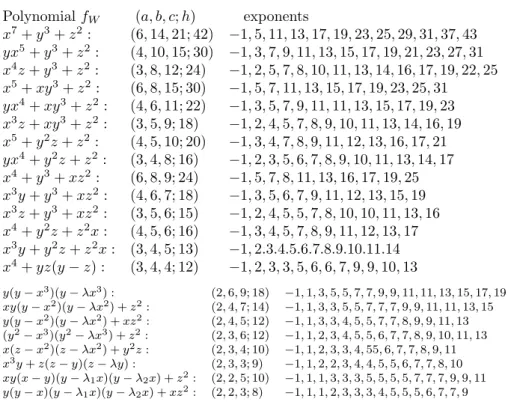
The singularities associated with the 14 weight systems with εW =−1 are
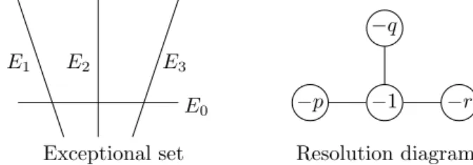
called exceptional uni-modular singularities by Arnold [Ar3]. Certain distin-guished bases of the lattices of vanishing cycles for them have been calculated by Gabrielov ([Gab2], see Table 12), where the triplet (p,q,r) of lengths of the three branches of the diagram is called the Gabrielov number. On the other hand, the exceptional set of the minimal resolution of the 14 singularities is given by a star-shape configuration of 4 rational curves (see Table 11), where the triplet (p,q,r) of the minus of the self-intersection numbers of the three branching curves is called the Dolgachev number. Then Arnold observed that there is an involutive one to one correspondence from the set of 14 exceptional uni-modular singularities to itself, which exchange the Gabrielov number and the Dolgachev number. The involution is called the strange duality ([Ar3],§13). The strange duality, which is nowadays understood as an appearance of mirror symmetry3, admitted several interpretations. Among these, in§14, we
introduce ∗-duality on regular systems of weights, which is an involution ∗ on a set of regular systems of weights and is characterized as follows: let us recall the characteristic polynomial ϕW(λ) :=Qµi=1(λ− exp(2π
√ −1mi
h)) ∈ Z[λ] of the
2As in simple Lie algebra case, the symplectic structures on the co-adjoint orbits of the
elliptic Lie group are expected to form a primitive form. See [Sa14] VI (Integrable Highest Weight Modules), VII (Elliptic Groups and their Invariants), in preparation, and [Ya3]).
3The reader is referred to [Kon],[Yau] for mirror symmetry in general and to [K-Y][Ta1]
for the Landau-Ginzburg orbifold case. Already in case of εW = 0, the algebraic data, i.e. the elliptic curve in the exceptional set in the resolution of the singularity, is not “mirror dual” to the elliptic root system of vanishing cycles obtained topologically. In order to get mirror symmetry here, one should think of the elliptic curve with a group action [Ta1]. A more comprehensive description is obtained by considering the pairs of a regular weight system and a group action [KST3]. However, in the present paper, we do not get into such details.
Coxeter element for W and decompose it asϕW(λ) =Qi|h(λi−1)eW(i). Then, W∗
is the∗-dual of W if and only if h=h∗ and eW(i) + eW∗(h/i) = 0 for all i∈Z>0
with additional conditions.4 We observe that any weight system with εW = 1
is selfdual; W = W∗, and that the ∗-duality induces the strange duality on the set of 14 weight systems with εW =−1. Therefore, we expect in general that
the∗-duality exchanges the algebraic approach for a weight system W with the topological approach for the dual system W∗. Then, instead of naive study of resolution diagrams of the singularity XW,0 in the algebraic side of W , what
stands for the basis of vanishing cycles of XW∗,0 in the topological side of W∗?
Inspired by the recent studies on mirror symmetry in mathematical physics ([K-L 1,2],[H-W],[Wal], see§15), we study the homotopy category HMFgrA
W(fW)
of matrix factorizations of the polynomial fW as the algebraic approach.5 We
devote§16 to three different descriptions of this category and its general proper-ties. We expect that the advantage of this approach is that the category carries a “universality” such that it recovers all the three approaches to the Lie algebra, which we have discussed above.6 Let us observe and explain this fact in the case
of the category for simple singularities with εW= 1, studied in§17.
We show that the category HMFgrA
W(fW) for εW=1 is generated by a strongly
exceptional collection (§16 4.), whose associated quiver is a Dynkin quiver ~∆ of type W , and that the path-algebraC~∆ is isomorphic to the algebra consisting of morphisms among the objects of the exceptional collection. Therefore, we have the equivalence HMFgrA
W(fW)'D
b(mod-C~∆) due to a theorem of
Bondal-Kaplanov (see §16 4). Hence, using the classical result by Gabriel [Ga], the lattice and the set of vanishing cycles for the weight system W = W∗ can be recovered by the K-group of the category and the set of indecomposable objects of the category, respectively. That is, HMFgrA
W(fW) recovers all three data for the
Lie algebra, discussed above, inducing the natural isomorphisms gW'g0W'g00W.
In the case εW=−1, the category HMFgrAW(fW) is generated by a strongly
exceptional collection whose associated quiver ∆A is given in Table 14, where
A is the signature set (13) of W (Footnote 32). We show again the equivalence HMFgrA
W(fW)'D
b(mod-C(∆
A, R)), whereC(∆A, R) is the quotient of the
path-algebra C∆A by the relation R (see (32)and §18 Theorem). Hence, in the 14
uni-modular exceptional cases, comparing Table 12 with 14 and in view of the strange duality, we conclude that the K-group of the category is isomorphic to the lattice of vanishing cycles for the∗-dual weight system W∗, as expected.
We expect further that the image set in the K-group of exceptional inde-composable objects of the category coincides with the set of vanishing cycles for the singularity XW∗,0, and, hence, the three approaches to the Lie algebra are
available from the category. Whether the three Lie algebras gW, g0W and g00W
for them are isomorphic to each other or not is an interesting open problem.
4The∗-dual W∗of W may not exist for all W, but is unique if it exists [Sa17]. It seems interesting to extend the concept of regular systems of weights (by considering group actions (Footnote 3) and non-hypersurface singularities), which is closed under the∗-duality.
5This was proposed by Takahashi [Ta2] (c.f. Orlov [Orl1]) answering a problem posed by
the author [Sa15] (5.3) Problem.§16, 17 and 18 are based on the joint works [K-S-T 1-2].
6It is also remarkable that the stability condition space [Br1][H-M-S] on the category seems
1
Simple Polynomials
There are a finite number of regular polyhedra, namely, the icosahedron, do-decahedron, octahedron, hexahedron and the tetrahedron, known at the time of Platon. The regular dihedron, which has only two faces of the n-gon (n≥ 3), is nowadays included in the list of regular polyhedra. The subgroup G of SO(3) consisting of rotations of three dimensional Euclidean space, which moves a reg-ular polyhedron (centered at the origin) to itself, is called the regreg-ular polyhedral group. The binary extension ˜G of the regular polyhedral group G is obtained by taking the inverse image of G through the surjective homomorphism SU (2)→ SO(3). It is well-known that the binary regular polyhedral groups (including bi-nary dihedral groups) and the cyclic subgroups Zn:=
¿µ exp2π √ −1 n 0 0 exp „ −2π√−1 n « ¶À for n∈ Z>0 together form a complete list of finite subgroups of SU (2) up to
conjugacy. As an abstract group, all of the groups have a presentation: hp, q, ri := h x, y, z | xp= yq = zr= xyzi
for suitable integers p, q, r∈ Z>0, given in the next Table 1 (here, x, y and z
induces the rotation of the polyhedron centered at an edge, a face and a vertex).
Table 1.
h1, b, ci ' Zn ' cyclic group of order n = b + c
h2, 2, ni ' D2n ' binary dihedral group of n-gon n ≥ 2
h2, 3, 3i ' A4 ' binary regular tetrahedral group
h2, 3, 4i ' S4 ' binary regular octahedral group
h2, 3, 5i ' A5 ' binary regular icosahedral group
In fact, these are the only cases when the grouphp, q, ri is finite (see [C-M]). The group is sometimes called the Kleinean group because of the following result due to A. Schwarz [Sc] and F. Klein [Kl1].
Theorem. Let ˜G ⊂ SU(2) be a Kleinean group. Let it act linearly on C2,
and, hence, on the ringC[u, v] of polynomial functions on C2 (where u, v ares
coordinates ofC2). Then the subringC[u, v]G˜:={P ∈ C[u, v] | gP =P ∀g∈ ˜G}
of invariants is generated by 3-homogeneous elements, say x, y and z, which satisfy a single relation, say fG˜= f (x, y, z). That is:
C[u, v]G˜' C[x, y, z]/(f ˜ G).
The polynomial fG˜ is called a simple polynomial, which is listed below.
Table 2.
Type fG˜ Kleinean group
Al xl+1+ yz Zn
Dl x2y + y1−1+ z2 h2, 2, ni
E6 x4+ y3+ z2 h2, 3, 3i
E7 x4+ xy3+ z2 h2, 3, 4i
E8 x5+ y3+ z2 h2, 3, 5i The Types in the left-side shall be explained in§3.
F. Klein, in the introduction to his lecture notes on the icosahedron [Kl1], described the time when he and Lie studied together in Berlin and Paris during the years 1869-70: “At that time we jointly conceived the scheme of investigating geometric or analytic forms susceptible of transformation by means of groups of changes. This purpose has been of directing influence in our subsequent labors, though these may have appeared to lie far asunder. Whilst I primary directed my attention to groups of discrete operations, and was thus led to the investigation of regular solids and their relations to the theory of equations, Professor Lie attacked the more recondite theory of continued groups of transformations, and therewith of differential equations”.
2
Simple Lie algebras and root systems
Let us explain another stream of mathematics started from Lie and Killing. The Lie algebras describe “the infinitesimal structure of continuous groups”. The series of works [Ki] by Killing starting from the year 1888, determining the structure of simple Lie algebras, (which was completed by E. Cartan [Ca]) has introduced a new mathematical structure (see [Ha]) which goes far beyond the class of simple Lie algebras, and is strongly influential on the present program. Killing looked at the adjoint action of the abelian (Cartan) subalgebra of a simple Lie algebra and decomposed the algebra into a direct sum of equi-eigenspaces of the action. Since an equi-eigenvalue (as an element of the dual space of the Cartan subalgebra) is a root of the characteristic equation, he called it a root (Wurzel), and showed that the system of roots for a simple Lie algebra satisfies some properties, which are now known as the axioms for a finite root system (see ([Bou]§6no1)). The classification of simple Lie algebras is reduced
to the classification of finite root systems. In fact, it is achieved by determining the matrix (2I(α, β)/I(α, α))α,β∈Γ(called the Cartan matrix), where I is Killing
form and Γ is a simple basis of the root system7.
3
Du Val diagrams and Coxeter diagrams
Let us see how the two streams of mathematics, one starting with Klein and the other with Lie-Killing, meet again in the year 1934, when Du Val and Coxeter were together at Trinity college in Cambridge. At that time, the concept of the Weyl group, generated by reflections sα for all roots α of the Lie algebra, was
established in connection with the representation theory of simple Lie algebras (Weyl [We] (1925-6) and Cartan [Ca]). The classification of root systems is
7Recall [Bou](chap.6§1 5.) that a simple basis of a (finite) root system is characterized
as a system of linear forms on the Cartan algebra, whose zeros define the system of walls (oriented to the inside) of a Weyl chamber. It is admirable that, even at such an early stage (1888) of the study of simple Lie algebras, Killing ([Ki]S12,13) began to study root basis Γ, the productQα∈Γsα of the reflections sα associated to the basis (presently known as the Coxeter-Killing transformation) and its eigenvalues (which presently defines the exponents). However, for their geometric significance in terms of the Weyl group and chambers, one must wait until Weyl’s work [We]. As we shall see, finding generalizations of the simple root basis, Coxeter- Killing transformations and the exponents are central problem in the present paper.
reduced to the classification of the Weyl group [Wae]. Then Coxeter, by use of the fundamental domain (=Weyl chamber) of the Weyl group, classified all finite reflection groups acting on Euclidean space. Namely, he gave an explicit presentation of the Weyl group in terms of generators and relations, known as the Coxeter relations [Co1].8 He introduced a diagram (tree) Γ, where the vertices correspond to the generators and an edge is drawn between two vertices which are non-commutative (see [Bou] for more details on reflection groups). In Table 3, the Coxeter’s diagram for the Weyl groups of types Al, Dl, or El are
given by removing i) the vertex ρ0 of the diagram and ii) the “tilde e ” from
the types in RHS of table (see Appendix for more details on the table).
Table 3.
Kleinean group Diagram Type
ρ
0ρ
ρ
0ρ
ρ
0ρ
ρ
ρ
0ρ
0ρ
Z
nh2, 2, ni
h2, 3, 3i
h2, 3, 4i
h2, 3, 5i
˜
A
n−1˜
D
n+2˜
E
6˜
E
7˜
E
8The complex hypersurface X0 in C3 defined by the zero-loci of a simple
polynomial in the list of Klein (Table 2) has an isolated singular point at the origin 0 (cf.§11 Fact4.), called a simple singularity [Dur]. In the year 1934, Du Val [Du] studied the (minimal) resolution π : ˜X0→ X0of the simple singularity.
He associated a diagram Γ to the resolution: decompose E := π−1(0) into irreducible components∪l
i=1Ei, then, vertices xi of the diagram are in one to
one correspondence with components Ei and an edge is drawn between xi and
xj if Ei∩ Ej 6= ∅. He observed that for each Kleinean group on the LHS of
Table 3, the diagram he obtained is exactly the one given in the middle of the Table 3, deleting the vertex ρ0. In the introduction of [Du], he wrote “It may
be noted that the “trees” of curves which we have had to consider bear a strict formal resemblance to the spherical simplices whose submultiple of π, considered by Coxeter”. In the same volume of the London Journal, Coxeter [Co1] listed diagrams for reflection groups following a request of Du Val. (For the definitions of diagrams for a basis of a lattice, see Footnote 41, and for a quiver, see§16, 6) .)
8The generators are given by the reflections attached to the walls of the chamber (which
is bijective to the set Γ of simple basis of Killing) and the relations are given by the dihedral group relations for every pair of generators along 2-codimensional facets of the chamber. The higher codimensional facets of the chamber do not play a role in determining the group.
4
Brieskorn’s Description of the universal unfolding
We observed in §3 that there is a one to one correspondence between the dia-grams of Du Val associated to simple polynomials and those of Coxeter in the classification of simple Lie algebras (recall Table 3). However, at this stage, their relation remained a “strict resemblance”, as Du Val wrote. A more direct and decisive relationship was found 40years later in the work of Brieskorn and Grothendieck. In ICM Nice 1970, Brieskorn [Br4] reported the following result. Theorem. (Brieskorn [Br4]) Let X→ S be the universal unfolding9of a simple
singularity, and let g be the corresponding simple Lie algebra. Then, one has a commutative diagram:
X ⊂ g
↓ ↓
S ' g//Ad(g) ' h//W
where i) the vertical arrow in right side of the diagram is the adjoint quotient morphism due to Chevalley’s theorem, and ii) X⊂ g is an embedding of X onto a transversal slice to the nilpotent subvariety of g at a subregular element.
Brieskorn further described the simultaneous resolution (c.f. [Br1,2]) of the universal family.10 He wrote “Maybe the two theories do not lie so far asunder”.
Remark 1. The Brieskorn’s description of the universal unfolding X→ S of a simple singularity by use of a simple Lie algebra has the advantage in determin-ing certain global differential geometric structures on the family, since, in the Lie algebra, the integrability conditions are already built in. For instance, the primitive form of the family X→ S11, which is defined by an infinite system
of non-linear equations, for the simple singularity is described by the Kostant-Kirirov symplectic form [Sa7] [Yah] [Ya1] [Yo]. The flat structure (Frobenius mfd structure) on the deformation parameter space S is described by the Coxeter-Killing transformation of the Weyl group [Sa16] [He] [Sab].
These facts motivated the author to convince the following: for a further class of singularities, using suitable Lie algebras, construct primitive forms and flat structures globally. However, the list of regular polyhedral groups and that of the simple Lie algebras have already been used up. Are these the only cases where singularity theory and Lie theory come happily together?
9The concept of an unfolding of a singularity of a function f is due to R. Thom [Th].
We shall give in §5 and in Footnote 12. a brief description of them. From an algebraic geometric view point, it is essentially the same concept as a semi-universal deformation of the hypersurface defined by f = 0 near at the singular point ([?], [Sch] and [Tu]).
10This was reproven by a use of representation of quivers [Kr] (see the works by H. Nakajima
for further studies on the relationship between Lie algebras and representations of quivers).
11For a primitive form, see [Mat][Od1][Sa7][Sa19]. It is a relative de-Rham cohomology
class ζ∈ HDR(X/S) which 1) generates all the other de-Rham cohomology classes as aDS -module, and 2) satisfies an infinite system of bi-linear differential equation (by means of residue pairings). Its local existence on S is known [Sai]. Global existence on S is known only for simple or simply elliptic singularities. It is believable that g is the Cartan prolongation of
X with respect to the primitive form. Such global construction of primitive forms by means
of globally defined integrable systems (such as Lie algebras) is the basic motivation in the present paper. However, we shall not discuss the primitive form itself in any further detail.
5
Universal unfolding of a Hypersurface Singularity
Before we go further, we prepare some terminologies on vanishing cycles of a hypersurface isolated singular point studied by authors [Br3] [Le1] [Gab1] [Eb1]. Let f (x) with x := (x0,· · ·, xn) (n≥ 0) be a holomorphic function defined in
a neighborhoodU of the origin 0 of Cn+1 with the coordinate x. Assume that the hypersurface X0:={(x)∈U | f(x)=0} has an isolated singular point at the
origin 0∈X0. This is equivalent to that Jf:=C{x}/ “∂f (x) ∂x0 ,· · · , ∂f (x) ∂xn ” is of finite rank overC, where C{x} is the local ring of all convergent series in x.
Theorem. (Milnor [Mi]) Consider a map f : X→ Dε where X :={x ∈ U |
|x| < δ} ∩ f−1(Dε) and Dε:={t ∈ C | |t| < ε} for positive real numbers δ, ε such
that 0 < ε << δ << 1. Then, f|X\f−1(0) : X \ f−1(0) → Dε\ {0} is a locally
trivial topological fibration such that the general fiber is homotopic to a bouquet of µf-copies of n-sphere Sn, where µf := dimCJf is called the Milnor number.
The fibration is called the Milnor fibration, whose general fiber, denoted by X1, is called the Milnor fiber. If f is globally defined weighted homogeneous
polynomial of positive weights, then we may choose δ = ε =∞.
As a consequence of this result, the (reduced) homology group of the Milnor fiber is non-trivial only in dimension n, and we have ˜Hn(X1,Z)'ZµW.
Let us introduce particular elements of ˜Hn(X1,Z), called vanishing cycles:
let us consider a universal unfolding of f (Thom [Th]), which is a function F (x, t) in x∈Cn+1 and t = (t
1,· · · , tµf)∈C
µf defined in a neighborhood of the
origin (0, 0)∈ Cn+1×Cµf satisfying i) F (x, 0) = f (x), and
ii) ∂F (x,0)∂t
i (i = 1,· · · , µf) span theC-vector space Jf.
For a small value of t, again by choosing δ and ε suitably for ft(x) = F (x, t),
we consider the map ft: X→Dεsuch that, excluding finite number of its fivers
over the critical values, it gives a locally trivial fibration, whose general fiber is homeomorphic to the Milnor fiber. If t is general, then ft|X has exactly µf
-number of non-degenerate critical points and the (critical) values are distinct (i.e. ftis a Morsification of f ). We may choose the “base point” 1 whose fiber
ft−1(1) is the Milnor fiber X1on the boundary of the disc Dε. Let g : [0, 1]→Dε
be any continuous path starting at 1 and ending at a critical value c, without passing any critical points on [0, 1). Then the pull-back X[0,1] of the fibration
X → D² over the interval [0, 1] retracts to Xc. Thus, the natural inclusion
X1⊂ X[0,1] induces a homomorphism ι : ˜Hn(X1,Z) → ˜Hn(Xc,Z) whose kernel
ker(ι) is rank 1 (since the Hessian of ftat the critical point is non-degenerate).
Definition Let the setting be as above. Any base e∈ ker(ι) (up to sign) of the kernel in ˜Hn(X1,Z) is called a vanishing cycle along the path g. We denote by
Rf the set of all vanishing cycles running the path g and the critical values c.
Let γ be a path in Dεwhich starts at 1 and move along g close to the critical
value c and then turns once around c counter-clockwisely, and then return to 1 along g. This path induces the monodromy ρ(γ)∈ Aut(˜Hn(X1,Z)), whose
action on u∈ ˜Hn(X1,Z) is described by the following Picard-Lefschetz formula:
ρ(γ)(u) = u− (−1)n(n−1)2 (u, e)e
homology group (Footnote 35). If n is even, it is symmetric and (e, e) = (−1)n/22 so that ρ(γ) is a reflection action with respect to the vector e, denoted by we.
• • • 1 cµf ci c1 γ • • • • • • • γ1 gi gµf γµf g1 Table 4. .
Now, we describe the distinguished basis of the middle homology group ˜Hn(X1,Z), depending on two
choices: i) to give a numbering of the critical values, say c1,· · · , cµf, of ft, ii) to choose µfpaths g1,· · · , gµ
in Dεsuch that a) each giis a path connecting 1 with
ci as above, which is not self-intersecting, b) distinct
paths giand gj are intersecting only at 1, and c) the
passes g1,· · · , gµ are starting at the point 1 in the
linear order 1, . . . , µf counter-clock wisely (Table 4).
Fact-Definition. Under the above the setting, the set e1,· · ·, eµf of vanishing
cycles (up to choices of sign) associated to the paths g1,· · ·, gµf form an ordered
basis of ˜Hn(X1,Z), called a distinguished basis ([Br3], [Le1], [Gab1], [Eb1])
Monodromy. Let γ be the path starting at 1 turning once around the bound-ary of Dε counter-clock wisely and comes back to 1. The monodromy of this
path c := ρ(γ)∈ Auto(˜Hn(X1,Z)) is called the Milnor monodromy. Since γ is
homotopic to the product γ1· · · γµf of paths γi (see Table 4), we express c:
c = we1· · · weµf
as a product of reflections associated to a distinguished basis e1,· · · , eµf.
• • • • g1 gi+1 gµf • gi cµf c1 1 Table 5. .
Braid group Bµf action on distinguished
ba-sis: First, we remark that the homotopy classes of the paths γ1,· · · , γµf give a free generator
sys-tem of the group π1(Dε\{c1,· · ·, cµf}, 1). Thus the
choice of the paths g1,· · ·, gµf, up to homotopy,
cor-responds to a choice of the generator system of the free group. On the other hand, the braid group Bµf
acts on the set of free generator systems, as usual: for 1≤ i < µf, define an action σi : γ1,· · · , γµf 7→
γ1,· · · , γi−1, γiγi+1γi−1, γi, γi+2,· · · , γµf. This causes an action of σi on paths
g1,· · · , gµf to those given in Table 5. and on the distinguished basis e1,· · · , eµf
to e1,· · · , ei−1, wγi(ei+1), ei, ei+2,· · · , eµf. One can immediately verify that σi
(1≤i<µf−1) satisfy Artin braid relations (see [Ar]) so that we obtain a braid
group action on the set of distinguished basis.
Remark 2. Even if we start with a globally defined weighted homogeneous poly-nomial f of positive weights, in order to construct the fibration ft : X → Dε
above, we need to shrink the domain of ftsuitably by a use of δ and ε as above.
In fact, the embedding of a Milnor fiber Xtinto the global affine surface ˆXt:=
{x ∈ Cn+1| F (x, t) = 0} induces a non-trivial extension ˜H
n(Xt,Z) ⊂ ˜Hn( ˆXt,Z),
if one of the coordinate ti has negative weight (c.f. §11,b),4)). The extension is
generated by vanishing cycles “coming from∞” and is expected to play key role in analytic theory of primitive forms (see [Sa19]§6 Conjecture and Problem I’). Remark 3. In mathematical physics, hypersurface singularity is studied under the name Landau-Ginzburg model.
6
Simply Elliptic Singularities
We return to the main stream of our considerations in the present paper: to seek for a connection of primitive forms with Lie theory.
In the year 1974, the author [Sa2] came up with a new class of normal surface singularities, which are “located on the boundary” of the deformation space of simple singularities. They are called the simply elliptic singularities, which include the following three types of hypersurfaces:
Table 6 T ype equation fW E· E (µ+, µ0, µ−) ˜ E6 or E (1,1) 6 x3+ y3+ z3+ λxyz −3 0, 2, 6 ˜ E7 or E (1,1) 7 x4+ y4+ z2+ λxyz −2 0, 2, 7 ˜ E8 or E (1,1) 8 x6+ y3+ z2+ λxyz −1 0, 2, 8
The simple elliptic singularities X0are characterized from two different view
points: a) by the resolution of the singularity X0: a normal singular point 0 of a
surface X0is simply elliptic if and only if, by definition, the minimal resolution
π : ˜X0→ X0 of the singularity contains only a single elliptic curve E = π−1(0),
and b) by deformation of the singularity: a singular point 0 of a hypersurface surface X0 is either simple or simply elliptic if and only if any singularity in a
local deformation of X0 admits a weighted homogeneous structure.12
Here, a) the resolution diagram in the sense of Du Val consists only of a single elliptic curve E and it is hard to find Lie theoretic data, in contrast with
12Let us explain what do we mean by 1. “singularity in a local deformation of X
0”, and 2.
“weighted homogeneous structure” on a singularity X0.
X
ϕ 0 1 C Xϕ(x) Cϕ Dϕϕ
S
ϕ 0 x X1X0 C3ϕ
Local deformation of X0 .1. Recall §5 the universal unfolding F (x, t) defined in a neighborhood ˜U of the origin of Cn+1× Cµf. Then, it defines
a local analytic flat family of analytic varieties ϕ :Xϕ→ Sϕ where Xϕ:={(x, t) ∈ ˜U | F (x, t) = 0}, Sϕ:=Cµf and ϕ is the projection to the second factor. The fiber ϕ−1(0) over 0 is nothing but the original singular surface X0so that the family
{Xt:= ϕ−1(t)}t∈Sϕ is called the semi-universal deformation
of the singularity in X0 ([K-S],[Sch]). One can show that the
critical set Cϕ of the map ϕ is (locally near at 0) a smooth subvariety of dimension µf− 1, which is finite over Sϕso that the image Dϕ:= ϕ(Cϕ) is (locally near at 0) a hypersurface in
Sϕ, called the discriminant of ϕ. Then, for any point x∈ Cϕ, the variety Xϕ(x)= ϕ−1(ϕ(x)) is singular at the point x. This is a singularity in a local deformation of X0. As we saw already,
for a generic point x∈ Cϕ, (Xϕ(x), x) is an ordinary double point (i.e. Morse singularity). 2. Let X0be a hypersurface in a neighborhood of the origin 0 ofCn+1defined by an analytic
equation f (x) = 0 with an isolated singular point at 0. We say that X0 admits a weighted
homogeneous structure at 0 if there is a local analytic coordinate change at 0 such that the defining equation f (x) is transformed to a weighted homogeneous polynomial P (x) (i.e. P (x) = P
a0i0+···anin=hci0···inx
i0
0 · · · x
in
n for some positive integers a0,· · · , an and h). Then, the following i), ii) and iii) are equivalent [Sa1]: i) X0admits an weighted homogeneous structure,
ii) The sequence: 0→ C → OX0,0 d → Ω1 X0,0→ · · · d → Ωn+1 X0,0→ 0 is exact, where (Ω·X0,0, d) is the de Rham complex over X0at 0, and iii) f belongs to the ideal
“∂f (x) ∂x0 ,· · · , ∂f (x) ∂xn ” in the local ringC{x}.
the case of the simple singularity. However, b) they show a new and immediate relation (in a symbolical level) with Lie theory through deformation theory as follows: in the local deformation (see 1. of Footnote 12) of an elliptic singularity of type ˜Γ∈ { ˜E6, ˜E7, ˜E8}13, only an elliptic singularity of the same type ˜Γ or a
simple singularity can appear. The simple singularity of type Γ can appear if and only if Γ is a subdiagram of ˜Γ. This fact was explained soon after by use of the lattice (H2(X1,Z), I) (here, I = −(·, ·), see Footnote 35).14 Thus, for a
simply elliptic singularity X0, a relationship with Lie theory begun to appear
from the lattice of the smoothing X1, instead of the resolution ˜X0. Do we need
to change our view point? 15 We shall come back to this question of “change
of view-points” later when we discuss∗-duality in §14 and 15.
7
Vanishing cycles for simple and simply elliptic singularities
In order to sharpen the new view point, i.e. to study the lattice (H2(X1,Z), I) of
the middle homology group of the smoothing X1of singular surface X0, we
con-sider a particular subset R⊂H2(X1,Z), the set of vanishing cycles introduced in
§5 (c.f. [Sa15](5.2),(5.3)). From this view point, let us state some consequences of Brieskorn’s description [Br4] on simple singularities:
1) The minimal resolution ˜X0 and the smoothing X1of a simple singularity X0
of type Γ are homeomorphic. Hence one obtains an isomorphism of lattices:
∗) H2(X1,Z) ' H2( ˜X0,Z) .
Here, the homotopy type of the homeomoprhims, and hence the isomorphism ∗) depend on the Weyl group of type Γ. In fact, the ambiguity of the isomor-phism can be resolved (up to an outer automorisomor-phism of the Weyl group) by choosing the base point 1 in the totally real region (see Footnote 16).
2) The set of vanishing cycles R in H2(X1,Z) (see §5) forms a finite root system
of type Γ, and H2(X1,Z) is identified with the root lattice QΓ of the root system.
3) The homology classes [Ci]∈ H2( ˜X0,Z) (i = 1,· · ·, l) of the exceptional curves
in the resolution ˜X0are mapped by the homomorphism∗) to a simple root basis
Γ of the root system R, which are also distinguished basis in the sense in§5.16
If X0 is a simply elliptic singularities, none of 1), 2) or 3) holds. However,
2) suggests to regard the set of vanishing cycles in H2(X1,Z) for a Milnor fiber
13The names ˜E
iare taken from that of the affine Coxeter diagrams (Table 3) for the reason explained in this section. They are nowadays called also Ei(1,1)for the reason in the next§7.
14This is shown by using the fact that the lattice (H
2(X1,Z), I) is isomorphic to QΓ˜⊕ Z
(see [Ga], [Eb1,2]) where QΓ˜ is the affine root lattice of a type ˜E6, ˜E6 and ˜E8. See next§7. 15This question is supported by the fact that the period domain for the period mapRζ of
the primitive form is determined from the lattice H2(X1,Z) [Sa7]. 16The paths g
1,· · ·, gµf in Sϕ (Footnote 12), with whom associated distinguished basis
e1,· · ·, eµf is the simple root basis, is given in [Sa20]§4.3 Figure 6. and Theorems 4.1 and
4.2, using semi-algebraic geometry of the real discriminant Dϕ,Rof the universal deformation of the simple singularity. Furthermore, the associated paths γii = 1,· · ·, µ (Table 4) generate the fundamental group π1(Sϕ\ Dϕ, 1) and satisfy Artin braid relations of type Γ so that the fundamental group becomes an Artin group ([Br5] [B-S]). Then, the intersection matrix (I(ei, ej))ij=1,···,µis shown to become the Cartan matrix of type Γ by solving the braid relations
X1 of an elliptic singularity as a generalization of root systems. In fact, we can
generalize the root systems17 by removing the finiteness axiom from [Bou] so that the set of vanishing cycles for any even dim. hypersurface isolated singu-larity becomes a generalized root system. In particular, the set of vanishing cycles for a simply elliptic singularity is characterized as an elliptic root system, that is, a root system belonging in a semipositive lattice with radical of rank 2 ([Sa14]). However, by the lack of 1) and 3), we cannot find a generalization of “the simple root basis” of the elliptic root system naively from the resolution of X0. Also, no geometric method to choose one particular distinguished basis (§5)
is knowm.18 However, we choose some root basis arithmetically19such that the
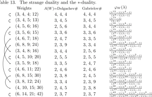
elliptic Coxeter-Killing transformation defined as a product of reflections asso-ciated with the basis is of finite order. Elliptict diagrams (see Footnote 41 for a definition of a diagram) associated to the basis are given in Table 7.
Table 7. Simply laced Elliptic diagrams of Codim=1 ([Sa14] I, Table 1).
1
3
6
0
5
4
3
2
1
4
2
The numbers attached at vertices are the exponents of the root system (see §7).
4
3
2
1
2
1
2
3
0
E
7(1,1)E
8(1,1)1
2
3
2
1
1
2
0
1
1
0
1
1
2
E
6(1,1)D
4(1,1)The diagrams plays basic role, as in the finite root system case, in describ-ing the elliptic root systems [Sa14]I, elliptic Weyle groups [ibid]III, elliptic Lie algebras [S-Y]. The construction of the primitive forms is a work in progress.20
17A subset R of a real vector space equipped with a symmetric form I is called a (generalized)
root system ifZR is a full lattice, 2I(α, β)/I(β, β)∈Z and α−2I(α, β)/I(β, β)β∈R for ∀α, β ∈R, and irreducible in a suitable sense ([Sa14]I). A root system is finite or affine if I is positive definite or semidefinite and rank(radical)=1, respectively. A root system is called elliptic if I is positive semidefinite and rank(radical)=2. The set of vanishing cycles for a simply elliptic singularity of type ˜E6, ˜E7 or ˜E8 is the elliptic root system of type E(1,1)6 , E
(1,1) 7 or E
(1,1) 8 . 18Gabrielov [Gab2] (Fig. 10 and 11.) obtained the diagrams in Table 7. for certain
distin-guished basis as one of the possible choices after the braid group action under the guiding principle to find the diagrams containing small number of triangles. On the other hand, in the simple singularity case, the semialgebraic geometry of the discriminant ([Sa20]) can yield the distinguished basis which corresponds to the simple root basis of the finite root system (see also A’Campo’s [AC]). There seems a gap between topology and semi-algebraic geometry.
19There does not exist elliptic Weyl chambers and, hence, there seemed no a priori definition
of a simple basis for an elliptic root system (see [Klu]). However, the elliptic diagram in Table 7. is defined by duplicating the vertex of the affine diagram at the largest exponent (see [Sa14]I(8.6)). We define the elliptic Coxeter-Killing transformation ceas the product of reflections (acting on H2(X1,Z)) attached to the vertices of the elliptic diagram (in a suitable
order). Then one has: i) ce is of finite order h, and the eigenvalues of ce determine the exponents of the elliptic root system (see§8 and Table 9), ii) the eigenvector of cebelonging to the eigenvalue 1 is regular in the elliptic Cartan algebra hewith respect to the elliptic Weyl group Weand iii) the universal central extension ˜Weof Weis generated by a lift ˜che. Using i), ii) and iii), a flat structure on the quotient space ˜he// ˜Weis constructed ([Sa15]II, [Sat,1,2]).
8
Exponents and Weight Systems
In this section, we first introduce the exponents for a finite or elliptic root system, which play important role in the classical and elliptic Lie theory21. Then, we try
to extend the definition of exponents for a generalized root system, and meet with a problem of “choice of the phases”. This fact leads us to introduce a new concept: the regular system of weights.
First, we recall a definition of exponents for a finite or elliptic root system. In both cases, define a Coxeter-Killing transformation as a product c, in a suitable order, of reflection actions on the lattice H2(X1,Z) attached to a simple root
basis (recall§5). The c is of finite order h (called the Coxeter number, see §19 Re-mark)22. Then the exponents m
1,· · ·, mµ are integers such that exp(2π
√ −1mi
h)
(i = 1,· · ·, µ) are the eigenvalues of c (see [Bou]Ch.v,no6.2 and [Sa14] I (9.7)
Lemma A.iii)). However, this determines only the exponents modulo h. In case of finite root systems and elliptic root systems, one poses further the constraint on the range 0≤mi≤h and on the symmetricity mi+mµ−i+1= h. Under these
constraints, we determine uniquely their exponents as in the next tables.
Table 8.
Type (a, b, c; h) exponents
Al(l≥ 1) (1, b, c; l + 1) 1, 2, . . . , l (b+c = l+1) Dl (l≥ 3) (2, l−2, 1−1; 2(l−1)) 1, 3, 5, . . . , 2l − 3, l − 1 E6 (3, 4, 6; 12) 1, 4, 5, 7, 8, 11 E7 (4, 6, 9; 18) 1, 5, 7, 9, 11, 13, 17 E8 (6, 10, 15; 30) 1, 7, 11, 13, 17, 19, 23, 29 Table 9
Type (a, b, c : h) exponents
E6(1,1) (1, 1, 1 : 3) 0, 1, 1, 1, 2, 2, 2, 3 E7(1,1) (1, 1, 2 : 4) 0, 1, 1, 2, 2, 2, 3, 3, 4 E8(1,1) (1, 2, 3 : 6) 0, 1, 2, 2, 3, 3, 4, 4, 5, 6
by vertex operators [Bo1] for all elliptic real roots, b) an algebra generated by the Chevalley triplets attached to the elliptic diagram (Table 7) satisfying the generalized Serre relations, and c) an amalgamation of an affine algebra and a Heisenberg algebra. An algebra isomorphic to any one of them is called an elliptic algebra. It is also a universal central extension of a 2-toroidal algebra. We remark that the elliptic root systems and the Lie algebras are found also from the representation theory of tubular algebras (see Y. Lin and L. Peng [L-P,1&2]). Works on highest weight representations and Chevalley type invariants for an elliptic algebra and group are in progress. Due to the above existence of the regular element, several properties similar to classical algebraic groups and its invariant theory hold for the elliptic Lie algebras and its adjoint groups. These facts supports the program that the elliptic primitive forms are constructed on the elliptic Lie algebras (see references in Footnote 2).
21The exponents give the degrees of basic g- or W -invariants and play basic roles in Lie
theory (see [Ko],[Sp],[St1]), and also in the study of the flat structures ([Sa16],[Sa14]II,[Sa7]).
22The Coxeter-Killing transformation has distinguished properties: i) c is of finite order h,
ii) the primitive hth roots of unity (or, 1 for an elliptic root system) are eigenvalues of c, and the eigenvectors of c belonging to them are regular (i.e. they are not fixed by the Weyl group and the adjoint group of the Lie algebra, [Col], [Bou] chap.V§6 no2, [Sa14]II§10 Lemma B). This existence of regular eigenvectors is basic for the construction of the adjoint quotient mor-phism g→g//Ad(g) ' h//W ([Ko],[Sp],[St1]) and of the flat structure on h//W ([Sa16],[Sa14]).
We intend further to introduce the exponents through Coxeter-Killing tr. (Milnor Monodromy) for root systems of singularities (since they are necessary data for primitive forms; see discussions below). In fact, we shall obtain in§18 quite interesting class of generalized root systems of Witt index 2 together with some distinguished root basis. However, we meet here a subtle problem: range of exponents, which lead the author to introduce the concept of the weight system. To explain the problem concretely, we cite some results from later sections.
1. Consider a polynomial in LHS of Table 10 in§13, whose zero loci defines a hypersurface X0 inC3with an isolated singular point at the origin.
2. The generalized root system (= the set of vanishing cycles) in H2(X1,Z)
in the middle homology group of a Milnor fiber X1of X0has a root basis in the
diagram Table 12 (where p, q, r, called the Gabrielov#, are given in Table 13). 3. Define the Coxeter-Killing transformation c as the product of reflection actions on H2(X1,Z) of the vertices of the diagram in a suitable order. Then,
c is of finite order h and the characteristic polynomial of c is given in the form (15) for a system of integers mi called exponents given in Table 10.
4. Observes that mi’s in Table 10 is exceeding the interval [0, h]. Thus, the
Coxeter-Killing transformation is unable to determine their phases (:= [mi/h])
for these new class of root systems. On the other hand, these mi/h without the
ambiguity “modulo 1” are well defined directly from a primitive form.23
Concern: The root system with basis may not have sufficient data to deter-mine the phases of exponents and to construct the primitive forms.
We shall discuss again on this issue. See§14 Remark 7. This fact, due to the important role of exponents [Sa7][Sai], leads the author to handle them directly (but not through eigenvalues of Coxeter-Killing transformation) as follows.
Consider the generating function24of exponents in Tables 8 and 9. (1) χ(T ) := Tm1+ Tm2+· · · + Tmµ.
Then, marvelously, the generating functions of the exponents for the finite and elliptic root systems of types Al, Dl, E6, E7, E8 and E
(1,1) 6 , E (1,1) 7 , E (1,1) 8 have a
decomposition25 of the form:
(2) χ(T ) = T−h(T
h− Ta)(Th− Tb)(Th− Tc)
(Ta− 1)(Tb− 1)(Tc− 1)
where a, b, c are integers and h is the order of the Coxeter element c such that (3) 0 < a, b, c < h and gcd(a, b, c) = 1.
Note that the weights a, b, c are uniquely determined from the function χ(T ), except for the type Ah−1.26 See Tables 8 and 9 for explicit lists of (a, b, c; h). The
23The proportions m
i/h are eigenvalues of an operator N in the flat structure associated to the primitive form, and are called exponents of the flat structure ([Sa4][Sa7] (3.3) Definition).
24It is introduced as the Fourier transform of the distribution of the exponents [Sa4] (3.1.1)
[Sa7] (3.3.14) in order to study the distribution of the zero-loci of χ.
25In the present paper, we are interested in only the cases when all roots of χ(T ) = 0 are
on the unit circle. But, this is not the case in general for a general primitive form (see [Sa4]).
26The characteristic function for the type A
h−1is expressed as χAh−1(T ) = T +· · ·+Th−1= Th−T
T−1 = T−h (T
h−T )(Th−Tb)(Th−Tc)
generating function (1) of exponents for a finite or an elliptic root system are characterized by the factorization (2) as follows. Consider abstractly a system:
(4) W := (a, b, c; h)
of 4 integers satisfying (3) (and additionally, a = 1 if b+c = h called type Ah−1),
and call it a weight system (a, b, c the weights and h the Coxeter number). Fact 1. ([Sa11]Theorem 2) If the function χW (2) for W has no poles, then it is
equal to a generating function (1) of exponents either for a finite root system of type Al, Dl, E6, E7, E8 or for an elliptic root system of type E
(1,1) 6 , E (1,1) 7 , E (1,1) 8 .
Let us call the rational function χW:= χ in (2) the characteristic function
associated to W , and call a weight system W is simple (resp. elliptic) if its characteristic function χW is equal to a generating function (1) for a finite root
system (resp. elliptic root system) (explicitly, see Table 8 and 9). 27
Before analyzing the characteristic function χW further, we state another
fact, which gives a meaning to the weights a, b, c and to the Coxeter number h in case of a simple and elliptic weight system (see Table 2 and 4 for a proof): Fact 2. A simple polynomial fG˜(x, y, z) in Table 2 (resp. an equation for an
elliptic singularity in Table 6) is a weighted homogeneous polynomial of degree h with the weights a, b, c on the variables x, y, z for a simple (resp. elliptic) weight system (a, b, c; h). The simple weight system determines the simple polynomial, up to a homogeneous coordinate change, uniquely. The elliptic weight system determines the equation up to one parameter (=the modulus of elliptic curves).
9
Triangle ∆ of Weight System, Geometry and Algebra
Summarizing the results of previous sections, we obtain the following triangle among three mathematical objects: weight system, geometry and algebra:
{ Simple weight systems }
(5) ⇓ ⇑
©
Kleinean groups ª⇒ ½
Simple Lie algebras with simple root basis
¾ . Here, the three arrows are construed as follows.
1) The correspondence ⇒ (denoted by Φ⇒) is given in three different ways (depending on the view points), all of which give the same result:
a) Use the Du Val diagram for the simple singularity (§1 and 2) and obtain the diagram of the simple root basis of the simple Lie algebra,
b) Use the set of vanishing cycles for the singularity (§5) and obtain the set of real roots of the simple Lie algebra,
c) Use the McKay correspondence ([Mc], see Appendix) and obtain the
27To be exact, one should add the diagram for D(1,1)
4 (recall Table 7.) in the list. A diagram
is called simply-laced if it does not contain a multiple edges. Any other diagrams for simple (or, elliptic) root system is obtained by the foldings of these simply-laced diagrams.
Dynkin graph for the simple Lie algebra.
Here, a) and b) are equivalent due to Brieskorn’s theorem (recall§7 1),2) and 3)). c) gives the dual basis of the basis given by a) with respect to the Killing form (see Appendix), but is more direct algebraic construction.
2) The correspondence ⇑ (denoted by Φ ⇑) is given by the decomposition (2) of the generating function (1) of the exponents (Table 7) of the root system. 3) The correspondence ⇓ (denoted by Φ⇓ ) is given by the pair of the funda-mental group π1(X0\ {0}) for the hypersurface X0 defined by the polynomial
in Table 2 and its action to the covering space ˜X0 (use Fact 2, c.f. [Mu1]).
By a direct inspection of the cases, we see that a composition of the three arrows Φ ⇓ , Φ⇒ and Φ ⇑ starting at any corner of the triangle (5) is an
iden-tity.28 Here we stress that the key step among the three arrows is the horizontal
correspondence Φ⇒. The others are rather straight forward. As a consequence of this observation, we conclude that
The datum of the set of exponents for a finite root system, which, a priori, is a very small part of the information of the root system, is sufficient to recover the root system and the simple Lie algebra. In the same way, the datum of a system W of weights (4) is sufficient to reconstruct the simple Lie algebra.
A similar triangle as (5) holds for the triple of elliptic weight systems, Heisen-berg groups of rank 2 ([Sa14] II, Appendix) and elliptic Lie algebras ([Sa14] IV). This supports the construction of the elliptic primitive forms and the flat struc-tures from the elliptic Lie algebras (still in progress). This motivates the author to generalize the triangle by starting with a wider class of weight systems.
We propose to use the top corner of the triangle as follows: consider any weight system W (4) of 4 integers. Then, relaxing the condition on χW(T ) (2)
to be a polynomial to to be a Laurent polynomial, we extend the class of weight systems and then look for some geometric objects in the left corner and some algebras in the right corner, respectively. That is: we try to recover the triangle:
{ Weight system W }
(6) ⇓ ⇑
{Geometry of XW} =⇒ {Algebra gW}
where the goal of the triangle is to construct primitive forms and their associated period mappings and automorphic forms (see [Sa19] for the details on the goal). Actually, without this setting of the goal, the objects and the correspondences in the triangle (6) are ambiguous (see§12). Note that each corner of the triangle is not a category and the correspondences⇒,⇓ and ⇑ are not functors. However, we expect a sort of “functoriarity” (yet to be defined) due to the deformation relations among XW’s.
28A similar triangle is obtained by replacing the three corners by{elliptic weight systems},
{Heisenberg groups of rank 2 with the extension classes -3,-2,-1} and {Elliptic Lie algebras of
10
Top corner of the triangle: regular systems of weights
We start with recalling the definition [Sa11] of a regular system of weights.29 Definition. A weight system W = (a, b, c; h) (4) is called regular if the charac-teristic function χW(T ) := T−h
(Th−Ta)(Th−Tb)(Th−Tc)
(Ta−1)(Tb−1)(Tc−1) belongs toZ[T, T−1].
In the following Fact 3 and in Fact 4 in the next section, we give two basic properties of a regular system of weights. The two properties are equivalent to the definition of the regular systems of weights, and they already attribute to the properties in the right and left corners of the triangle (6), respectively.
We first discuss about the new definition of exponents.
Fact 3.([Sa11]Theorem 1) A weight system W (4) is regular, if and only if there exist integers m1,· · · , mµ with µ = µW=(h−a)(h−b)(h−c)abc called the rank of
W , such that χW (2) is developed into the sum of monomials of the form (1).
We call m1,· · · , mµ the exponents of W30, which we order: m1≤ · · · ≤ mµ
linearly. By use of the functional equality ThχW(T−1) = χW(T ), one has the
duality of exponents:
(7) mi+ mµ−i+1 = h (i = 1,· · · , µ).
A fact which is not used in the present paper but shall be of basic importance (see Footnote 22, ii)), is that there exists always an exponent prime to h [Sa,13,18]. The advantage to start from a weight system is that the exponents are a priori defined without an ambiguity of their phases (i.e. [mi/h] ∈ Z). The
smallest exponent min{m1,· · ·, mµ} is given and denoted by
(8) εW := a + b + c− h.
Actually,§8 Fact 1. implies that if εW> 0 (resp. = 0), then automatically one
has εW= 1 and W is a simple (resp. elliptic) weight system, whose exponents
coincide with the exponents of the corresponding finite or elliptic root system. For each negative integer ε < 0, there always exist a finite number of regular systems of weights having ε as the smallest exponent (e.g. W = (1, 1, 1; 3−ε), see [Sa12, Sa17] Appendix 1,2. for many interesting examples of W with εW < 0).
In particular, there exist 14+8 regular systems of weights for the case εW=−1
having no 0 exponents (see Table 10), on which we shall discuss more in details in the present paper.
We are now to analyze the other corners of the triangle (6). Recall that the finite or elliptic root system cannot be directly constructed from the weight system, but we needed to turn the triangle (5) counter-clockwisely. Similarly, we start with analyzing the left corner of (6) in the next section.
29This is slightly modified ([Yas]) from the original definition [Sa11]: χ
W(T ) has a pole at most at T = 0. Using a relation: Thχ
W(T−1) = χW(T ), the two definitions are equivalent.
30In order to agree with the classical convention in Lie theory (e.g. [Bou]), we have called
the integers mi exponents. However, from a view point of the flat structure on Sϕ (recall Footnote 23), one should better call the rational numbers mi/h exponents. This view point becomes important again, when we consider the category of graded matrix factorizations§16.
11
Left corner of the triangle: a geometry of X
WFinding the objects in the left corner and Φ ⇓ of the triangle (6) follows from the following characterization Fact 4. of the regularity of a weight system W .
For any given W = (a, b, c; h), consider a weighted homogeneous polynomial
(9) fW(x, y, z) :=
P
ai+bj+ck=hcijkxiyjzk.
Fact 4. ([Sa11]Theorem 3) The weight system W (4) is regular, if and only if there exists a polynomial fW of the form (9) such that the quotient ring:
(10) JW := C[x, y, z]/ ³ ∂fW ∂x , ∂fW ∂y , ∂fW ∂z ´ ,
called the Jacobi ring of fW, is of finite rank µW overC (“if” part is trivial).
Actually, any polynomial (9) with generic coefficients carries this property. In fact, Fact 4. is trivially equivalent to that the hypersurface
(11) XW,0 := {(x, y, z) ∈ C3| fW(x, y, z) = 0}
has an isolated singular point at the origin, i.e. XW,0 is smooth except at the
origin 0∈ XW,0, due to the Nullstellensatz of Hilbert.
Let us call fW in Fact 4. a polynomial of type W . We employ the polynomial
fW, or the hypersurface XW,0 (11) with the isolated singular point at 0 and
admitting a good C×-action31 λ∈ C× : (x, y, z) 7→ (λax, λby, λcz) on it as for
the object in the left corner of the triangle (6). Following the history described in§2-7, we analyze XW,0 from two: a) algebraic and b) topological view points.
a) Orbi-bundle K
1
εW
CW over the curve CW.
There are many studies on surface singularities with a goodC×-action (e.g. [Dol1,2,3,4], [Pin4,5], [Sa11,12,16], [Wa,1,2]). We recall a few results of them, which are necessary in our purpose. First, we remark that the smoothness of X0\{0} implies that the quotient variety
(12) CW := (XW,0\ {0})/C× = Proj(C[x, y, z]/(fW(x, y, z))
is a smooth curve. However, theC×-bundle XW,0\{0}C
×
→ CW has some finite
number of singular fibers (i.e. fixed by some non-trivial finite subgroups, called isotropy groups, ofC×). In this sense, CW carries also a structure of an orbifold
curve (to be precise, an algebraic stack). The pair (g : p1,· · · , pr) of the genus
g of the curve CW and the signature set of the orders of the isotropy groups:
(13) A(W ) = {p1,· · · , pr}
is called the signature of the orbifold ([F-K]pp.182-190). In fact, we have Fact 5. ([Sa11]Theo.6) The genus g of the curve CW is equal to the multiplicity
a0 := #{1 ≤ i ≤ µ | mi = 0} of exponents equal to 0. The set A(W ), up to
some pi= 1, is explicitly determined from the weights W arithmetically.32
31The action is said good since the the exponents of the action a, b, c are positive (or,
equivalently, the coordinate ring RW :=C[x, y, z]/(fW) is positively graded.
32The genus and the signature set of the orbi-curve C
![Table 7. Simply laced Elliptic diagrams of Codim=1 ([Sa14] I, Table 1).](https://thumb-ap.123doks.com/thumbv2/123deta/5797782.1530131/14.892.233.624.456.599/table-simply-laced-elliptic-diagrams-codim-sa-table.webp)