RIMS-1675
Folder complexes and multiflow combinatorial dualities
By
Hiroshi HIRAI
July 2009
RESEARCH
INSTITUTE FOR
MATHEMATICAL
SCIENCES
Folder complexes and multiflow combinatorial dualities
Hiroshi HIRAI
Research Institute for Mathematical Sciences, Kyoto University, Kyoto 606-8502, Japan
July 2009
Abstract
In multiflow maximization problems, there are several combinatorial duality re-lations, such as Ford-Fulkerson’s max-flow min-cut theorem for single commodity flows, Hu’s max-biflow min-cut theorem for two-commodity flows, Lov´asz-Cherkassky duality theorem for free multiflows, and so on. In this paper, we provide a unified framework for such multiflow combinatorial dualities by using the notion of a folder
complex, which is a certain 2-dimensional polyhedral complex introduced by Chepoi.
We show that for a nonnegative weight µ on terminal set, µ-weighted maximum mul-tiflow problem admits a combinatorial duality relation if and only if µ is represented by distances among certain subsets in a folder complex, and show that the corre-sponding combinatorial dual problem is a discrete location problem on the graph of the folder complex. This extends a result of Karzanov for the case of metric weights. Also we give a special optimality criterion to such combinatorial dual problems and give a characterization of such weights in terms of the combinatorial dimension.
1
Introduction
Let G be an undirected graph with nonnegative edge capacity c : EG → R+. Let
S ⊆ V G be a set of terminals. A path P in G is called an S-path if its ends belong to
distinct terminals. A multiflow is a pair (P, λ) of a set P of S-paths and its nonnegative flow-value function λ : P → R+ satisfying capacity constraint
P
P∈P:e∈P λ(P ) ≤ c(e)
for e∈ EG. For a nonnegative weight µ :¡S2¢→ R+on the set of pairs of terminals, the
µ-weighted maximum multiflow problem (µ-problem for short) is formulated as
Maximize X
P∈P
µ(sP, tP)λ(P )
(1.1)
subject to (P, λ) : multiflow for (G, c; S),
where sP, tP denote the ends of P . The µ-problem (1.1) is a linear problem. So there is
a linearly programming duality relation. However, for a special weight µ, the µ-problem admits a combinatorial duality relation. For example, suppose that S is a 2-set {s, t}. Then the µ-problem is the maximum flow problem. The max-flow min-cut theorem, due to Ford-Fulkerson [8], says that the maximum flow value is equal to the minimum s-t cut value. Suppose that S is a four-set {s, t, s0, t0}, and µ(s, t) = µ(s0, t0) = 1 and other weights are zero. Then the µ-problem is two-commodity flow maximization. Hu [14] proved that the maximum multiflow value is equal to the minimum of ss0-tt0 mincut value and st0-ts0 mincut value. Suppose that µ is all-one weight. Then Lov´asz [23] and Cherkassky [4] proved that the maximum multiflow value is equal to the half of the sum of t-S\ t mincut values over t ∈ S.
A remarkable result by Karzanov [17] completely characterized metric-weights µ admitting such a combinatorial duality relation. We shall describe it. Here µ is called a
metric if µ satisfies the triangle inequality. An undirected graph Γ is called a frame if
(i) Γ is bipartite,
(ii) Γ has no isometric cycle of length greater than four, and
(iii) Γ is orientable in the sense that Γ has an orientation with the property that, for each 4-cycle C, nonadjacent edges have opposite directions with respect to a cyclic ordering of C; see the left of Figure 4.
We denote the shortest path metric of Γ by dΓ.
Theorem 1.1 ([17]). Let µ be a metric on a finite set S. Suppose that there exist a
frame Γ and a map φ : S→ V Γ such that
µ(s, t) = dΓ(φ(s), φ(t)) (s, t∈ S).
Then, for any capacitated graph (G, c) having S as terminal set, the maximum value of the µ-problem (1.1) is equal to the minimum value of the following discrete location problem on Γ : Minimize X xy∈EG c(xy)dΓ(ρ(x), ρ(y)) (1.2) subject to ρ : V G→ V Γ, ρ(s) = φ(s) (s∈ S).
(Karzanov [17] presented this theorem in the dual form, i.e., the minimum 0-extension
problem on a frame is solvable by its metric relaxation, which is the LP-dual to the
metric-weighted maximum multiflow problem.) Moreover, if a rational metric µ can-not be represented by (a dilation of) a submetric of a frame, then there is no such a combinatorial duality relation [18]. From the point of the view in Theorem 1.1, Lov´ asz-Cherkassky duality relation can be understood as follows. Let µ be the all-one distance on S. Then 2µ is represented as the distance among the leaves of a star consisting of #S edges. A star is clearly a frame. Then (1.2) coincides with the problem of finding
t-S\ t mincut for each s ∈ S.
Unfortunately, this theorem cannot be applicable to µ-problems for nonmetric weights
µ, such as two-commodity flows. Our previous paper [11] partially extended Theo-rems 1.1 to a nonmetric version. However this result needs tedious calculations for the tight span and its subdivision, which cause difficulty and inconvenience for a further combinatorial study to µ-problems (1.1). The main contribution (Theorem 2.1) of this paper is a natural extension of Theorem 1.1 for general weights, which provides a useful and flexible framework for multiflow combinatorial dualities. Also this result is an im-portant step of the complete classification of weights µ having finite fractionality in the next paper [13].
To describe our result, we employee the notion of a folder complex (an F-complex for short) introduced by Chepoi [3, Section 7]. Roughly speaking, an F-complex is a 2-dimensional polyhedral complex obtained by filling a 2-dimensional cell into each
4-cycle of a frame. In Section 2, we describe basic definitions and the main result. A
key concept that we newly introduce in this paper is the notion of a normal set in an F-complex. Our main result (Theorem 2.1) says that if weight µ can be realized by the distances among normal sets in an F-complex under l1-metrization, then the µ-problem
has a combinatorial dual problem similar to (1.2). We also give illustrative examples for multiflow combinatorial dualities by F-complexes, including Karzanov-Lomonosov dual-ity relation for anticlique-bipartite commoddual-ity flows and seemingly new combinatorial duality relation for a weighted version of two-commodity flows.
Our main result immediately follows from two properties: one is the Helly property of normal sets, and the other one is a decomposition property of finite submetrics on an F-complex. This connection to Helly property sheds a new insight on the multiflow duality. To prove them, in Section 3, we reveal several intriguing properties of shortest paths connecting normal sets in an F-complex, which are previously known for shortest paths connecting vertices of a frame. These properties will also play key roles in the next paper [13]. In Section 4.2, we give a special optimality criterion to combinatorial dual problems, which extends one for the classical tree location problems. Also we verify that weight µ has such an F-complex realization if and only if µ has combinatorial dimension most 2. This result has already been suggested by the previous paper [11].
Notation. Let R and R+ be the sets of reals and nonnegative reals, respectively. The
set of functions from a set V to R is denoted by RV. For p, q ∈ RV, p ≤ q means
p(x)≤ q(x) for all x ∈ V .
A function µ : S× S → R is called a distance on S if µ(s, t) = µ(t, s) ≥ µ(s, s) = 0 for s, t ∈ S. We regard a nonnegative weight on terminals as a distance. A distance
d on S is called a metric if d satisfies the triangle inequality d(x, z) ≤ d(x, y) + d(y, z)
(x, y, z ∈ S). For a metric d on S, the minimum distance between two subsets A and B is denoted by d(A, B), i.e.,
d(A, B) = inf
x∈A,y∈Bd(x, y).
We simply denote d({x}, A) by d(x, A). For a subset A ⊆ S and a nonnegative real r, the ball B(A, r) around A of radius r is defined as
B(A, r) ={x ∈ S | d(A, x) ≤ r}.
For an undirected graph G, the vertex set and the edge set are denoted by V G and
EG, respectively. An edge joining x, y ∈ V G is simply denoted by xy or yx. Let dG
denote the shortest path metric on V G with some specified edge-length. If no edge length is specified, then dG means the shortest path metric by unit edge-length. A subgraph
G0 of G is called isometric if dG0(x, y) = dG(x, y) for x, y ∈ V G0.
Let F ⊆ 2S be a set of subsets. We say “F has the Helly property” if every subset
F0 ⊆ F having pairwise nonempty intersection
A∩ B 6= ∅ (A, B ∈ F0)
has nonempty intersection \
A∈F0
A6= ∅.
A polyhedral complex ∆ is a set of polyhedra in some Euclidean space such that every face of σ∈ ∆ belongs to ∆, and the nonempty intersection of σ, σ0 ∈ ∆ is a face of both
σ and σ0. Let|∆| denote the underlying setSσ∈∆σ. A member in ∆ is called a cell. A k-dimensional cell is simply called a k-cell. A 1-cell is also called an edge. If an edge has
ends p, q, then it is also denoted by pq. A k-dimensional polyheral complex is simply called a k-complex. For our applications to the multiflow theory, we always assume that
(R
2, l
1)
square
triangle
hypotenuse
leg
κ
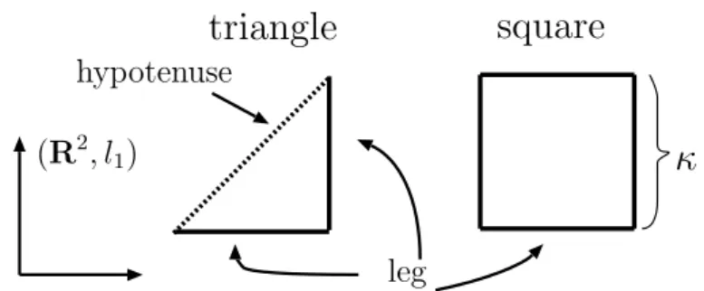
Figure 1: A square and a triangle equipped with the l1-distance
Figure 2: A folder
2
Definitions, results, and examples
Let ∆ be a (finite) 2-complex satisfying the following property:
(2.1) (i) For some positive rational κ, each maximal cell σ has an injective continuous map ϕσ : σ→ R2 such that the image ϕσ(σ) is
(a) the convex hull of{(0, 0), (κ, 0), (0, κ), (κ, κ)}, (b) the convex hull of{(0, 0), (κ, 0), (κ, κ)}, or
(c) the segment [(0, 0), (κ, 0)], and the image of a face of σ is a face of ϕσ(σ).
(ii) If σ∩ σ0 6= ∅ for two maximal cells σ, σ0, then ϕσ0◦ ϕ−1σ is an isometry from
ϕσ(σ∩ σ0) to ϕσ0(σ∩ σ0) in the Euclidean distance.
By condition (ii), if 2-cells σ, σ0 share a common edge e, then ϕσ(e) = [(0, 0), (κ, κ)]
implies ϕσ0(e) = [(0, 0), (κ, κ)]. An edge e of ∆ is called a hypotenuse if ϕσ(e) =
[(0, 0), (κ, κ)] for a 2-cell σ containing e. Other edge is called a leg. In particular, a maximal 1-cell is a leg. κ is called the leg-length. A 2-cell σ is called a square if its image by ϕσ is (a), and is called a triangle if its image by ϕσ is (b). Namely ∆ is obtained by
gluing squares and isosceles right triangles along same type of edges. A folder of ∆ is a square or the union of all triangles sharing one common hypotenuse; see Figure 2.
A more combinatorial and abstract approach is often useful. We can regard ∆ as a pair of a simple graph Γ0 and a subsetC of its chordless cycles such that
R
(a)
(b)
e
1e
2e
3F
1F
3F
2Figure 3: (a) violation of the flag condition, and (b) violation of the local convexity
(2.2) (i) the edge set of Γ0 is partitioned into two types of edges, called legs and
hypotenuses, and
(ii) each member ofC is
(a) a 3-cycle (a triangle) consisting of one hypotenuse and two legs, or (b) a 4-cycle (a square) consisting of four legs,
and every hypotenuse belongs to some triangle.
Indeed, we can take Γ0 as the 1-skeleton graph of ∆, and take C as boundary cycles of
2-cells. Conversely, from (Γ0;C) with property (2.2) and a positive rational κ, we can
construct a 2-complex ∆ with property (2.1).
We can endow |∆| with the lp-metric by the following way. For each cell σ and a
path P in σ, the lp-length of P is defined by the lp-length of ϕσ0(P ) in (R2, lp) for a
maximal cell σ0 containing σ (well-defined by (ii)). Then we can define the lp-length of
a path P in|∆| by the sum of the lp-length of P ∩ σ◦ over all cells σ, where σ◦ is the
relative interior of σ. Thus we can define the metric d∆,lp on |∆| by defining d∆,lp(p, q)
to be the infimum of the lengths of all paths connecting p, q in |∆|. In this paper, we are mainly interested in the l1-metrization d∆,l1, which is simply denoted by d∆.
A simply-connected 2-complex ∆ with property (2.1) is called a folder complex (an
F-complex for short) [3, Section 7] if
(2.3) (i) the intersection of any two folders does not contain incident legs, and (ii) there are no three folders Fi(i = 1, 2, 3) and three distinct legs ei(i = 1, 2, 3)
sharing a common vertex such that ei belongs to Fj exactly when i6= j.
In fact, this is equivalent to the condition that |∆| is a CAT(0) space under the l2
-metrization [3, Theorem 7.1]. We particularly call (ii) the flag condition; see Figure 3 (a). Next we introduce certain subsets of |∆|. A subset R of |∆| is called normal if it satisfies the following property:
(2.4) (i) R coincides with|K| for a connected subcomplex K of ∆ with the property that ifK contains a leg e, then every cell containing e belongs to K. (ii) there are no two triangles σ and σ0 sharing a leg and a right angle such that
Figure 4: Orientation
We particularly call (ii) the local convexity condition; see Figure 3 (b). Let Γ = Γ∆ be the graph consisting of all legs of ∆, called the leg-graph of ∆. Equivalently, Γ is the graph obtained by deleting all hypotenuses from the 1-skeleton graph of ∆. The edge-length of Γ is defined by κ uniformly. An F-complex ∆ is said to be orientable if the leg-graph Γ has an orientation such that
(2.5) (i) in each square, its diagonal edges have same direction. More precisely, orientations of two nonincident edges are opposite each other in a cyclic ordering of the corresponding 4-cycle, and
(ii) in each triangle, its right angle is neither a source nor a sink.
See Figure 4. In fact, the leg-graph of an orientable F-complex is a frame; see Theo-rem 3.2 in Section 3.1.
For a rational distance µ on set S, a pair (∆;{Rs}s∈S) of an F-complex ∆ and a set
{Rs}s∈S of normal sets is called an F-complex realization of µ if it satisfies
µ(s, t) = d∆(Rs, Rt) (s, t∈ S).
Namely, µ is realized by the l1-distances among normal sets Rs. Consider the µ-problem
(1.1) for a capacitated graph (G, c) with S⊆ V G, and consider the following continuous and discrete location problems on ∆:
Minimize X xy∈EG c(xy)d∆(ρ(x), ρ(y)) (2.6) subject to ρ : V G→ |∆|, ρ(s)∈ Rs (s∈ S). Minimize X xy∈EG c(xy)dΓ(ρ(x), ρ(y)) (2.7) subject to ρ : V G→ V Γ, ρ(s)∈ Rs∩ V Γ (s ∈ S).
Now we are ready to describe our main result.
Theorem 2.1. Let µ be a rational distance on S. Suppose that µ has an F-complex
realization (∆;{Rs}s∈S). Then, for any capacitated graph (G, c) with S ⊆ V G, the
following holds:
(1) The maximum value of the µ-problem (1.1) is equal to the minimum value of the
continuous location problem (2.6).
(2) In addition, if ∆ is orientable, then the maximum value of the µ-problem (1.1) is
Figure 5: 4-subdivision (a) (b) 1/2 Rs Rt Rs0 Rt0 R t0 Rs0 Rs Rt (R2, l 1) 1/2
Figure 6: Two-commodity F-complexes
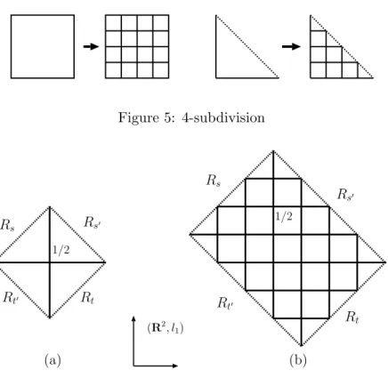
An F-complex ∆ may be not orientable. By the subdivision operation, we can always obtain an orientable F-complex as follows. For a positive integer k≥ 2, the k-subdivision
∆k is obtained from ∆ by subdividing each square into k2 squares, subdividing each
tri-angle into k(k−1)/2 squares and k triangles, and subdividing each maximal 1-cell(edge) into k edges as in Figure 5. The leg-length is set to be κ/k. One can easily see:
(2.8) (i) The k-subdivision ∆k is an F-complex for any k. (ii) The 2-subdivision ∆2 is always orientable.
Next we describe illustrative examples of combinatorial duality relations for µ-problems based on Theorem 2.1.
Two-commodity flows. First consider the case where terminal set S is a four-set
{s, t, s0, t0} and distance µ on S is given as µ(s, t) = µ(s0, t0) = 1 and others are zero.
Then the µ-problem (1.1) is the two-commodity flow maximization problem [14]. We can realize µ by the distance on an F-complex as follow. Consider four triangles, glue them around a common right angle, and define the leg-length κ to be 1/2, as in Figure 6 (a). The resulting 2-complex is clearly an orientable F-complex. Moreover ∆ realizes µ as the distance among four hypotenuses, which are normal. Theorem 2.1 (ii) gives a combinatorial duality relation for the two-commodity flow maximization.
Weighted two-commodity flows. Also we can consider a weighted version of two-commodity flows. Let µ be defined as (µ(s, t), µ(s0, t0)) = (p, q) for relatively prime positive integers p, q, and other distances are zero. Then consider an F-complex ∆ as in Figure 6 (b), which is a subdivision of a rectangle of edge-length ratio (p : q). Let κ = 1/2. Clearly ∆ is a F-complex. Again µ is realized by the distance of the
four edges of the rectangle, which are normal. Also one can see that ∆ is orientable. Then Theorem 2.1 (ii) yields a combinatorial duality relation, which seems new in the literature.
Anticlique-bipartite commodity flows. A 0-1 distance µ can be identified with a
commodity graph H on S by st ∈ EH ⇔ µ(s, t) = 1. We may assume that H has no
isolated vertices. The corresponding µ-problem for (G, c) is the maximization of the total sum of flow-values of multiflows connecting pairs of terminals specified by edges of H. For a multiflow f , the total flow-value with respect to H is denoted by kfkH. A
bipartition (X, Y ) of vertex set V G is called a cut, and its cut capacity c(X, Y ) is defined to be the sum of the capacity of edges with exactly one end belonging to X. A multicut
X = (X1, X2, . . . , Xk) (k≥ 2) with respect to H is a partition of V G with the property
that ends of each edge of H belong to distinct parts of X , and its capacity c(X ) is the sum of the capacity of edges whose ends belong to distinct parts of X . For a multiflow
f and a multicutX (w.r.t. H), the following obvious weak duality relation holds:
(2.9) kfkH ≤ c(X ).
In general, the duality gap is strict (except single- and two-commodity flows). Consider the following relaxation of multicuts. A semi-multicut X = (X1, X2, . . . , Xk) (k ≥ 2)
with respect to H is a set of disjoint subsets of V G with the property that ends of each edge of H belong to distinct sets in X , and its capacity c(X ) is defined as
c(X ) = 1 2 k X i=1 c(Xi, Xi).
Again the weak duality (2.9) holds for any multiflow and any semi-multicut, and the duality gap is still strict. However, the class of commodity graphs H admitting strong duality (for semi-multicuts) is not so narrow; recall Lov´asz-Cherkassky theorem for the case where H is a complete graph. Karzanov and Lomonosov [20] characterized such a class of commodity graphs H as follows.
Theorem 2.2 ([20]). Suppose that the setA of maximal stable sets of commodity graph
H has the following properties:
(1) For every triple A, B, C ∈ A of maximal stable sets, at least one of A ∩ B, B ∩ C,
and C∩ A is empty.
(2) The intersection graph of A is bipartite.
Then, for any capacitated graph (G, c) having H as commodity graph, the following holds:
max{kfkH | multiflow f} = min{c(X ) | semi-multicut X }.
See [22], and also see [9] for a polymatroidal approach to this result. A commodity graph with condition (1-2) is called anticlique-bipartite. Here we give an interpretation of this results in terms of an F-complex. Let us construct an F-complex realization for 0-1 distance µ corresponding to a commodity graph H with property (1). Let ΩA be the intersection graph ofA. From ΩA, we can construct an abstract 2-complex of (2.2). All edges of ΩA are supposed be hypotenuses. Add a new vertex O, and add a leg OA for each A ∈ A. Let Γ0 be the resulting graph. 2-cells C consists of 3-cycles of one
hypotenuse AB and two legs OA, OB over all intersecting pairs A, B ∈ A. Define the leg-length κ to be 1/2. Let ∆ be the resulting 2-complex, which is the join of O and
1
2
3
1
02
03
0(a)
R
1R
20R
30R
3R
2R
10(b)
O
1
02
03
011
0123
33
022
0 1/2Figure 7: (a) an anticlique bipartite commodity graph and (b) its F-complex realization
1/2
1/4
Figure 8: F-complexes for H = C5
ΩA. By the property (1), the girth of ΩA is at least four. This fact implies that ∆ is an F-complex; the violation of the flag condition at O implies the existence of a chordless cycle in ΩA of length at most three. For s∈ S, define a normal set Rs by
Rs=
½
hypotenuse AB if s belongs to exactly two A, B ∈ A, vertex A if s belongs to exactly one A∈ A.
Note that every terminal s belongs to at most two maximal stable sets by (1) and the assumption that H has no isolated vertices. Then (∆;{Rs}s∈S) is an F-complex
realization. Indeed, d∆(Rs, Rt) = 0 ⇔ Rs∩ Rt 6= ∅ ⇔ Rs∩ Rt ={A} for A ∈ A with
s, t ∈ A ⇔ µ(s, t) = 0, and Rs∩ Rt = ∅ implies that d∆(Rs, Rt) = 1. Furthermore ∆
is orientable if and only if the condition (2) is fulfilled. Consider the discrete location problem (2.7) for (∆;{Rs}s∈S). For a map ρ : V G → V Γ feasible to (2.7), the set
X := (ρ−1(A) | A ∈ A) is a semi-multicut, and P
xy∈EGc(xy)d∆(ρ(x), ρ(y)) coincides
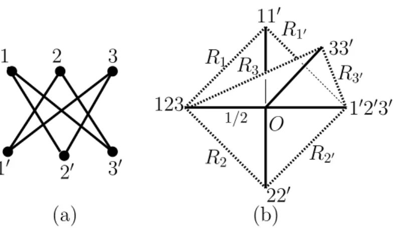
with c(X ). Thus Theorem 2.1 implies Karzanov-Lomonosov duality relation above. Figure 7 illustrates (a) an anticlique-bipartite commodity graph H of K3,3minus one
perfect matching, and (b) its F-complex realization ∆. In this case, ∆ is obtained by gluing six triangles of leg-length 1/2, and each Rs is a hypotenuse.
Also for nonorientable case, i.e., H violates (2), we obtain a combinatorial duality relation by subdividing ∆ into ∆2, which coincides with the one given in [16]. Figure 8 (a) illustrates an F-complex corresponding to the commodity graph of five-cycle, which is nonorientable, and (b) illustrates its 2-subdivision. See the next paper [13] for further examples.
3
Folder complexes and normal sets
Our main Theorem 2.1 is a consequence of the following two properties of an F-complex
∆; see the paragraph below.
(3.1) (i) For any collection of normal sets N1, N2, . . . , Nk and nonnegative rationals
r1, r2, . . . , rk, the collection of balls {B(Ni, ri)}ki=1has the Helly property.
(ii) Suppose that ∆ is orientable. For a map ρ : X → |∆| on a finite set X, define metric dρon X by
dρ(x, y) = d∆(ρ(x), ρ(y)) (x, y∈ X).
Then there exist maps ρi : X → V Γ (i ∈ I) such that dρ is a convex
combination of dρi and, for any normal set R, ρ(x)∈ R implies ρ
i(x)∈ R
(i∈ I).
(i) is an extension of [3, Theorem 7.8] for the case where each Ni is a singleton set; see
Section 4.2. The goal of this section is prove (3.1). In Section 3.1, we introduce some of basic notation. In Section 3.2, we study shortest paths connecting normal sets. By using them, in Section 3.3 we prove (3.1) (i). In Section 3.4, we show a certain decomposition property of shortest paths, and prove (3.1) (ii).
Proof of Theorem 2.1. Here we show Theorem 2.1 by assuming (3.1). The second statement (2) of Theorem 2.1 immediately follows from the first (1) and (3.1) (ii) (and (3.7)). So we show the first statement. Let µ be a rational distance on finite set S. For a capacitated graph (G, c) with terminal set S, consider the µ-problem (1.1). As is well-known [22], its LP-dual problem is given by
Minimize X xy∈EG c(xy)m(x, y) (3.2) Subject to m : metric on V G, m(s, t)≥ µ(s, t) (s, t ∈ S).
Let (∆;{Rs}s∈S) be an F-complex realization of µ. For a map ρ feasible to (2.6), define
metric dρ on V G as in (3.1) (ii). Then condition ρ(s)∈ Rs implies
dρ(s, t) = d∆(ρ(s), ρ(t))≥ d∆(Rs, Rt) = µ(s, t),
and thus dρ is feasible. Hence it suffices to show:
(3.3) For every rational metric m feasible to (3.2), there exists a map ρ : V G→
|∆| such that dρ≤ m and ρ(s) ∈ R
s for s∈ S.
The following argument is based on the idea used in [1, p.421]. Let m be a feasible rational metric. Let V G ={x1, x2, . . . , xn}. Define a map ρ : V G → |∆| recursively by
ρ(xk) being an arbitrary point in
(3.4) \ s∈S B(Rs, m(s, xk))∩ k\−1 i=1 B(ρ(xi), m(xi, xk)) (k = 1, 2, . . . , m).
We show that the set (3.4) is nonempty for all k, which implies that ρ is well-defined and satisfies ρ(s)∈ Rs and dρ ≤ m. Indeed, ρ(s) ∈ B(Rs, m(s, s)) = Rs, and ρ(xj) ∈
We use the induction on k. Suppose that (3.4) is nonempty for i < k. By ra-tionality, we can take ρ(xi) as a vertex of l-subdivision ∆l for large l. Then each
singleton set {ρ(xi)} is normal in ∆l. Of course, Rs is also normal in ∆l. By the
Helly property (3.1) (i), it suffices to show that each pairwise intersection is nonemtpy. Note that two balls B(R, r) and B(R0, r0) intersect if and only if d∆(R, R0) ≤ r +
r0. For s, t ∈ S, the nonemtpyness of B(Rs, m(s, xk))∩ B(Rt, m(t, xk)) follows from
m(s, xk) + m(xk, t) ≥ m(s, t) ≥ µ(s, t) = d∆(Rs, Rt). For s ∈ S and i < k, the
nonemtpyness of B(Rs, m(s, xk))∩B(ρ(xi), m(xi, xk)) follows from m(s, xk)+m(xk, xi)≥
m(s, xi)≥ d∆(Rs, ρ(xi)), where the last inequality follows from ρ(xi)∈ B(Rs, m(s, xi))
for i < k (by induction). For 1≤ i < j < k, the nonemtpyness of B(ρ(xi), m(xi, xk))∩
B(ρ(xj), m(xj, xk)) follows from m(xi, xk) + m(xk, xj) ≥ m(xi, xj) ≥ d∆(ρ(xi), ρ(xj)).
Thus we are done.
3.1 Preliminaries
Let Γ be an undirected graph. The interval IΓ(x, y) between x, y ∈ V Γ is defined to
be the set {z ∈ V G | dΓ(x, y) = dΓ(x, z) + dΓ(z, y)} (for some specified edge length).
An undirected graph Γ (with unit edge length) is called modular if for each triple x, y, z of vertices the intersection IΓ(x, y)∩ IΓ(y, z)∩ IΓ(z, y) is nonempty. An element in
IΓ(x, y)∩ IΓ(y, z)∩ IΓ(z, y) is called a median of x, y, z. A modular graph Γ satisfies
the so-called quadrangle condition:
(3.5) For any four vertices x, u, v, y with dΓ(x, u) = dΓ(x, v) = 1 and dΓ(u, y) =
dΓ(v, y) = dΓ(x, y)− 1, there exists a common neighbor w of u and v such
that dΓ(w, y) = dΓ(x, y)− 2.
Indeed, we can take w as a median of u, v, y.
A graph is called hereditary modular if all isometric subgraph is modular. Bandelt [2] gave an elegant characterization of hereditary modular graphs as follows.
Theorem 3.1 ([2]). A graph is hereditary modular if and only if it is bipartite and has
no isometric cycles of length greater than four.
Therefore a frame is just an orientable hereditary modular graph. Chepoi [3] estab-lished a relation between hereditary modular graphs and F-complexes. Here a folder consisting of a single triangle is called a triangle-folder.
Theorem 3.2 ([3, Theorem 7.1]). For a simply-connected 2-complex ∆ satisfying (2.1)
without triangle-folders, the following conditions are equivalent:
(i) ∆ is an F-complex.
(ii) its leg-graph Γ is a hereditary modular graph without K3,3 and K3,3− as induced
subgraphs.
In addition, (i)⇒ (ii) holds for any simply-connected 2-complex ∆ satisfying (2.1) (pos-sibly including triangle-folders).
K3,3− is the graph obtained from K3,3 by deleting one edge. Since both K3,3 and K3,3−
are nonorientable, the leg-graph of an orientable F-complex is a frame. We can partially reconstruct an F-complex ∆ from its leg-graph Γ based on the following property: (3.6) (i) every 4-cycle of the leg-graph Γ belongs to a (unique) folder.
(ii) every 3-cycle of the 1-skeleton graph of ∆, consisting of two legs and one hypotenuse, is the boundary of a triangle.
(i) follows from the argument in [3, Section 7]; this is not so obvious, which uses the simply-connectedness, CAT(0) property of ∆ under the l2-metrization, and the
Gauss-Bonnet Theorem. (ii) follows from (i). Indeed, the hypotenuse of 3-cycle belongs to some triangle. Use (i) for a possibly appearing 4-cycle of legs.
Therefore, if there is no folder consisting of at most two triangles, then ∆ is com-pletely reconstructed from its leg-graph; there are two ways splitting a square to two triangles. Moreover, for an arbitrary hereditary modular graph without K3,3 and K3,3−
as induced subgraphs, by filling a folder to each maximal complete bipartite graph K2,n
(n≥ 2), we obtain an F-complex without triangle-folders [3].
3.2 Geodesics
Here we investigate shortest paths connecting normal sets. Several important properties previously known for shortest paths connecting vertices can be naturally extended for shortest paths connecting normal sets.
Let ∆ be an F-complex. In this subsection, we assume that the leg-length κ is equal
to 1 for simplicity. We begin with:
(3.7) For normal sets N and M , we have d∆(N, M ) = dΓ(N∩ V Γ, M ∩ V Γ ).
Indeed, we can easily modify a (polygonal) geodesic between N and M so that it lies on the union of legs (as in the proof of [11, Proposition 4.2]). For notational simplicity, in the sequel we use the same d for d∆ and dΓ, and we denote IΓ(x, y) simply by I(x, y).
For a normal set R, let ΓR be the 1-skeleton graph of the subcomplex of ∆ induced by
R. The edge length of e of ΓR is defined to be 1 if e is a leg and 2 if e is a hypotenuse.
Lemma 3.3. For a normal set R, we have dΓR(x, y) = d(x, y) for x, y∈ V ΓR.
Proof. Suppose to the contrary that there are x, y ∈ V ΓR with dΓR(x, y) > d(x, y).
Take such x, y with dΓR(x, y) minimum. Then dΓR(x, y) ≥ 4. Indeed, dΓR(x, y) ≤ 2 is
clearly impossible. Suppose dΓR(x, y) = 3. Since Γ is bipartite, we have d(x, y) = 1
and therefore x and y are incident in Γ . Take a shortest path P connecting x, y in ΓR.
P∪ {xy} is a 3-cycle or a 4-cycle in 1-skeleton graph of ∆. In both cases, by (3.6) there
is a folder F containing P ∪ {xy}. Then R violates the normality (i) at F by xy 6⊆ R. A contradiction.
Take z ∈ IΓR(x, y) with min{d(x, z), d(z, y)} ≥ 2. By minimality assumption, we
have dΓR(x, z) = d(x, z) and dΓR(y, z) = d(y, z). Take a median w of x, y, z in Γ .
Then w 6∈ R. Take w0 ∈ I(z, w) incident to z (by a leg zw0). We show that there exists a triangle σ of vertices z, w0, u and hypotenuse zu such that u ∈ IΓR(z, x) and
σ ∩ R = zu. Then there also exists such a triangle σ0 for IΓR(z, y), and R violates
the local convexity in σ∪ σ0. Take x0 ∈ IΓR(z, x) incident to z. Suppose that x0z is a
leg. Then by the quadrangle condition (3.5) for z, x0, w0, x there exists x00 incident to x0 and w0 with d(z, x) = d(z, x00)− 2 and therefore there is a folder containing z, x0, x00, w0. By the normality (i), x00 must belong to R, and thus zx00 is a hypotenuse, and there is a required triangle σ having z, w0, x00. Suppose that x0z is the hypotenuse of some
triangle ˜σ having vertices x0, z, x0. By the quadrangle condition for z, w0, x0, x, there are
a common neighbor x00of x0 and w0with d(z, x00) = d(z, x)−2, and a folder F containing
z, w0, x0, x00. If x00 = x0, then ˜σ is a required triangle. So x00 6= x0. By the quadrangle
condition for x0, x0, x00, x we can find a folder F0 violating the flag condition at x0 with
˜
σ and F . A contradiction.
Lemma 3.4. For a normal set R and a leg e = xy, if e6⊆ R, then we have
d(R, x)− d(R, y) ∈ {−1, 1}.
Proof. Let T be the closure of a connected component of |∆| \ R. Since ∆ is
simply-connected, T ∩ R is connected. By the normality, T ∩ R consists of hypotenuses (or a single point). Therefore T ∩ R ∩ V Γ is contained by one color class of bipartite graph
Γ . The statement immediately follows from this fact.
The next lemma is an extension of the quadrangle condition (3.5). We also call it the quadrangle condition.
Lemma 3.5. For a triple x, u, v of vertices and a normal set R, suppose that d(x, u) =
d(x, v) = 1 and d(u, R) = d(v, R) = d(x, R)− 1.
(1) If d(x, R) = 1, then there exists a triangle σ of vertices x, u, v such that R∩σ = uv
(uv is a hypotenuse).
(2) If d(x, R) ≥ 2, then there exists a common neighbor w of u and v such that
d(w, R) = d(x, R)− 2.
Proof. (1). By Lemma 3.3, x and y are joined by a path P of length 2 in ΓR. Apply
(3.6) for cycle P ∪ {ux, uv}. (2). So suppose that d(x, R) = k ≥ 2. We use the induction on k. Take u0, v0 ∈ R satisfying d(u, u0) = d(v, v0) = k− 1 with d(u0, v0)(≤ 2k) minimum. Suppose d(u0, v0) = 2k. Then x ∈ I(u0, v0). Let u00 be a neighbor of u0 in
I(u0, x). By Lemma 3.3, we can take a vertex u01 ∈ IΓR(u0, v0) joined to u0 by a leg or a
hypotenuse in R. By repeated applications of the quadrangle condition (for u0, u00,·, v0
and for u00,·, ·, v0), as in the last part of the proof of Lemma 3.3, we can find a triangle σ of vertices u0, u00, u001 with R∩σ = u0u001 and d(v0, u001) = d(v0, u0)−2. Then d(u001, u) = k−1,
and this contradicts to the minimality assumption of (u0, v0).
So suppose d(u0, v0) < 2k. Take a median w∗(6= x) of u0, v0, x and take a neighbor w of x from I(x, w∗). If w = v, then by the quadrangle condition for x, u, v, u0 we can find a required vertex. Therefore w 6= u, v. By the quadrangle condition for x, u, w, u0, we can find a common neighbor u∗ of u, w with d(u∗, u0) = d(u∗, R) = k− 2. Similarly
we can find a common neighbor v∗ of w, v with d(v∗, v0) = d(v∗, R) = k− 2. If u∗= v∗, then we are done. So u∗ 6= v∗. Let F1 and F2 be the folders containing x, u, w, u∗ and
x, v, w, v∗, respectively. Apply the induction to quadrangle w, u∗, v∗, R. Then we can
find a folder F3 violating the flag condition at w with F1 and F2. A contradiction.
The next lemma is a certain convexity property of normal sets.
Lemma 3.6. Let M, N be two normal sets. For a vertex x∈ M, if d(x, N) > d(M, N),
then there exists an edge (leg or hypotenuse) xy⊆ M such that d(y, N) < d(x, N). Proof. Take a vertex w in M with d(w, N ) = d(M, N ). Since M is connected, we can
take a path P in ΓM connecting x and w. Among such paths, take P with the following
properties:
(a) the integration I of d(·, N) along P , i.e.,
I = X uv: leg in P d(u, N ) + d(v, N ) 2 + X uv: hypotenuse in P d(u, N ) + d(v, N ) is minimum.
(b) P contains legs as much as possible (under property (a)).
Let P = (x = x0, x1, . . . , xm= w). Define a sequence {ai}i=0,...,m by ai = d(xi, N ). We
show that{ai}i=0,...,m has no triple ai−1, ai, ai+1 with the property (i) ai−1= ai > ai+1
or (ii) ai−1 < ai> ai+1. This immediately implies the statement.
Case (i). Suppose to the contrary that ai−1 = ai > ai+1 holds for some i. By the
bipartite property, edge xi−1xi is necessarily a hypotenuse. By construction, there is a
triangle σ of vertices xi−1, xi, u such that u6∈ M. Also u 6∈ N. Suppose that xixi+1is a
leg. Then by the quadrangle condition for xi, xi+1, u, N , there are a common neighbor v
of xi+1, u and a folder F containing xi, xi+1, u, v. By normality, we have v ∈ M. Then
there is a triangle σ0 of vertices u, v, xi in F such that M violates the local convexity
at σ∪ σ0. A contradiction. Suppose that xixi+1 is a hypotenuse. There is a triangle σ
of vertices xi, xi+1, v such that v 6∈ M (by construction). If v = u, then M violates the
local convexity on σ∪ σ0. So v6= u. By the quadrangle condition for xi, v, u, N , there is
a common neighbor z(6= xi) of v, u and a folder F supported by xi, v, u, z. Again, by the
quadrangle condition for v, z, xi+1, N , there is a folder F0 violating the flag condition at
v with σ0 and F . A contradiction.
Case (ii). Suppose to the contrary that ai−1 < ai > ai+1 holds for some i. Then at
least one of xi−1xi and xixi+1is a hypotenuse. Otherwise, by the quadrangle condition
and the normality, the segment xi−1xi+1belongs to M . This contradicts to the
construc-tion. Suppose that both xi−1xi and xixi+1 are hypotenuses. Then there are triangles
σ, σ0 of vertices xi−1, xi, u and xi−1, xi, v (resp.) such that u, v 6∈ M. If u = v, then M
violates the local convexity on σ∪ σ0. Therefore u6= v. Also in this case, we can find a triple of folders violating the flag condition at u (or v) by repeated applications of the quadrangle condition, as above. Suppose that xi−1xi is a hypotenuse and xixi+1is a leg.
Then there is a triangle σ of vertices xi−1, xi, u with u6∈ M. Again repeated applications
of the quadrangle condition imply the existence of a triple of folders violating the flag condition at u. A contradiction.
From the proof, we obtain the following:
Lemma 3.7. Let M, N be two normal sets. For two distinct vertices x, y ∈ M with
d(x, N ) = d(y, N ) = d(M, N ), there is a hypotenuse xz in M with d(z, y) = d(x, y)− 2 and d(z, N ) = d(M, N ).
Next we discuss the extendability of a path to a shortest path connecting normal sets. Although our goal is Lemma 3.11 below, we derive it from a more general version (Lemma 3.9) for future applications in [13].
An F-complex ∆ is called star-shaped if there is a vertex p such that every folder contains p and no triangle contains p as its right angle. For a vertex p in ∆, let ∆p be
the subcomplex of ∆ consisting of cells containing p and their faces. Clearly ∆p is also
an F-complex. Although ∆p may not be star-shaped, (∆2)p is always star-shaped.
Lemma 3.8. Let p be a vertex, and let R be a normal set not containing p. Suppose
that ∆p is star-shaped. Then a point x in |∆p| at minimum distance from R is a vertex
and uniquely determined.
We call this vertex x the gate of R in ∆p; this definition is compatible to that in [7].
Proof. By p6∈ R and (2.4) (i), R does not contain a leg in ∆p. Since ∆p is star-shaped,
the boundary (relative to |∆|) consists of legs. By Lemma 3.4, the map x 7→ d(x, R) on a leg is monotone decreasing or increasing. Hence the minimum attains at a vertex. Suppose that two vertices x, y have the minimum distance from R. Consider the case
where x and y are not incident to p and have a common neighbor v (∈ ∆p). Then
x, v, p and y, v, p belong to folders F1 and F2, respectively. By the quadrangle condition
for v, x, y, R, we obtain a folder F3 violating the flag condition with F1 and F2. A
contradiction. Suppose other cases. Take a path P connecting x and y in ∆p passing
p. By applying the quadrangle condition for three consecutive vertices in P and R, we
find a vertex u in ∆p with d(u, R) < d(x, R), or a vertex z in ∆p with d(z, R) = d(x, R)
such that z and x have a common neighbor. The first case is clearly impossible, and the second case reduces to the case above for (x, z).
The extendability of a shortest path passing a vertex p can be locally characterized by the gates in ∆p (or (∆2)p when ∆p is not star-shaped).
Lemma 3.9. Let p be a vertex, and let M, N be normal sets not containing p. Suppose
that ∆p is star-shaped. Let x and y be the gates of M and N in ∆p, respectively. Then
the following two conditions are equivalent:
(1) d(M, N ) = d(M, x) + d(x, p) + d(p, y) + d(y, N ). (2) d(x, y) = d(x, p) + d(p, y).
Proof. (1) ⇒ (2) is obvious. We show the converse. We first consider the case where M is a singleton {w}. Our proof is based on that of [3, Lemma 7.6]. Suppose to the
contrary that d(w, N ) < d(w, x) + d(x, p) + d(p, y) + d(y, N ). We take such {w} with
k = d(w, x) minimum. Note that d(p, N ) = d(p, y) + d(y, N ) necessarily holds. Suppose
the case k = 0 (x = w). Suppose that x is incident to p. Then d(x, N ) = d(p, N )− 1. Take a neighbor z of p from I(p, y). Apply the quadrangle condition for p, x, z, N . Then we obtain a common neighbor u of x, z with d(u, N ) = d(z, N )− 1. Since u belongs to ∆p, we have z 6= y and d(x, y) = 3. Thus d(u, N) = d(y, N) and u 6= y, which
contradicts to Lemma 3.8. Suppose that x is not incident to p (d(p, x) = 2). Let z be a common neighbor of x and p. Then d(z, N ) = d(z, p) + d(p, y) + d(y, N ) by above. Thus d(x, N ) = d(z, N )− 1 holds. Apply the quadrangle condition for z, x, p, N. Then we obtain a common neighbor u of x and p with d(u, N ) = d(p, N )− 1. Then y is not incident to p, i.e., d(x, y) = 4. Take a common neighbor v of p and y. Apply the quadrangle condition for p, v, u, N . Then we obtain a common neighbor q of v, u with
d(q, N ) = d(y, N ). However q6= y by d(x, y) = 4. A contradiction to Lemma 3.8.
Suppose k = 1, i.e., w is incident to x. By the assumption and the bipartite property, we have d(w, N ) = d(x, N )−1. If x is incident to p, then by the quadrangle condition for
x, w, p, N there is a folder including w, p, x, and thus w belongs to ∆p. A contradiction.
Suppose that x is not incident to p. Take a common neighbor z of x and p. Then z, x, p belong to a common folder F1. Apply the quadrangle condition for x, w, z, N . We obtain
a common neighbor u of w and z such that d(u, N ) = d(w, N )−1. Then u, w, z, x belong to a common folder F2(6= F1). Apply the quadrangle condition for z, u, p, N . Then we
obtain a folder F3 violating the flag condition with F1 and F2. A contradiction.
So suppose k ≥ 2. Take a neighbor z of w from I(w, x), and take a neighbor u of z from I(z, x). Both gates of z and u in ∆p are x. By minimality assumption,
d(z, N ) = d(z, x) + d(x, p) + d(p, y) + d(y, N ). Therefore d(w, N ) = d(z, N )− 1. By
the quadrangle condition for z, w, u, N , there is a common neighbor r of w, u such that
d(r, N ) = d(z, N )− 2. Also the gate of r in ∆p is x and d(r, x) = d(w, x)− 1. Thus
d(r, N ) < d(r, x) + d(x, p) + d(p, y) + d(y, N ). A contradiction to the minimality of w.
Next we show that M is general. Suppose that (1) fails for k = d(M, x) = 0 (x∈ M). Suppose that x is incident to p. By Lemma 3.6 and the quadrangle condition, we can find a triangle such that its hypotenuse belongs to M and its right angle is p. This
contradicts to the fact that ∆p is star-shaped. Suppose that x is not incident to p.
Let z be a common neighbor of x and p. Let F be a folder containing z, x, p. By Lemma 3.6 and the quadrangle condition, we can find a triangle σ of vertices x, z, u such that xu = M∩ σ and d(u, N) = d(x, N) − 2. By the quadrangle condition for z, p, u, N, we can find a folder F0 violating the flag condition with F and σ. Suppose that (1) fails for k = d(M, x) > 0. Take w ∈ M with d(w, x) = d(M, x) such that d(w, N) is minimum. By the singleton case above, d(w, N ) = d(w, x) + d(x, p) + d(p, y) + d(y, N ) holds, and thus d(w, N ) > d(N, M ). By Lemma 3.6, there is z ∈ M incident to w by a leg or a hypotenuse such that d(z, N ) < d(w, N ). Let w0 ∈ I(w, x) be a neighbor of w. By repeated applications of the quadrangle condition, we can find a triangle σ of vertices w, w0, z0 such that w0z0 = σ∩ M and d(z0, N ) = d(w, N )− 2. Consider the
distance d(z0, x). Then d(z0, x) < d(w, x) contradicts to the definition of w. Therefore d(z0, x) = d(w, x) = d(M, x). However this contradicts to the minimality of d(w, N ).
By the same idea of the proof of Lemma 3.8, we have:
Lemma 3.10. For a folder F and a normal set R not meeting the interior of F , a point
x in F at minimum distance from R is a vertex and uniquely determined.
Also we call x the gate of R in F . Since F = |(∆2)p| for the center vertex p of the
2-subdivision of F , as a corollary of Lemma 3.9, we obtain the following fact, which is an extension of [17, p.87, Claim 3] for the case where N, M are singleton sets.
Lemma 3.11. Let F be a folder, and M, N normal sets not meeting the interior of F .
Let x and y be the gates of M and N in F , respectively. If x and y are not adjacent, then we have
d(M, N ) = d(M, x) + 2 + d(y, N ).
We also give a variant of Lemma 3.11; a proof is similar.
Lemma 3.12. Let M, N be normal sets, and let σ be a triangle with vertices x, y, z and
hypotenuse yz. Suppose that M∩ σ = yz and x is the gate of N in the folder containing σ. Then we have
d(M, N ) = 1 + d(x, N ).
3.3 Helly property of normal sets
The goal of this subsection is to prove:
Theorem 3.13. For an F-complex, the collection of normal sets has the Helly property.
In fact, (3.1) (i) is a simple corollary of it. For a ball B(N, r) for normal set N and rational radius r, we can subdivide ∆ into ∆k and further subdivide ∆k into ˜∆k by
splitting squares into two triangles so that B(N, r) is the union of a subcomplex of ˜∆k.
(3.8) B(N, r) is normal in ˜∆k.
Proof. Note that N is also normal in ˜∆k. Then (2.4) (i) immediately follows from the
bipartite property. Suppose to the contrary that there are adjacent two triangles σ, σ0 violating (2.4) (ii) with B(N, r). Let x be a common right angle of σ and σ0. Then
d(x, N ) = r + 1/k. Let y and z be distinct neighbors of x belonging to σ and σ0, respectively. Then d(y, N ) = d(z, N ) = r. By the quadrangle condition for x, y, z, N , we can find a folder F violating the flag condition at x with σ and σ0. A contradiction.
We prove Theorem 3.13 by extending Chepoi’s shelling argument in [3, p.157]. As Chepoi did, we will remove cells at the maximum distance from some vertex x. So we begin with studying the set
Mx= ½ y∈ |∆| ¯¯¯ d(y, x) = max u∈|∆|d(u, x) ¾ . It is easy to see:
(3.9) Mx is the union of isolated vertices and hypotenuses of triangle-folders.
Mx itself may not be normal.
(3.10) Any normal set M in Mx is a vertex or a tree consisting of hypotenuses.
Proof. We can regard M as a graph of hypotenuses. Suppose that M has a cycle C whose
vertices are ordered cyclically as (y0, y1, . . . , ym−1). Each edge yiyi+1 is the hypotenuse
of the unique triangle-folder σi. Here the indices are taken modulo m. Let y1i be the
right angle of σi. By normality, y1i 6= yi+11 for each i. By the quadrangle condition for
yi, yi1−1, y1i, x, there is a common neighbor yi2 of yi1−1, y1i with d(y2i, x) = d(yi, x)− 2 for
each i. If yi2 = y2i−1, then we obtain a triple of folders violating the flag condition at
y1i. Therefore yi26= yi−12 for each i. Again by the quadrangle condition for yi1, yi2, yi+12 , x,
there is a common neighbor yi3of yi1, yi+11 with d(y3i, x) = d(yi1, x)−2 for each i. Similarly y3
i 6= yi3−1 holds for each i. Repeat this procedure. Then d(y j
i, x) strictly decreases. In
the final step k = d(x, M ), we have yki = x for each i. Thus we obtain a triple of folders violating the flag condition at yik−1. A contradiction.
We are ready to prove Theorem 3.13. We use the induction on the size of ∆. Take some vertex x. Consider Mx and its connected components.
Case 1: Mx has a connected component of an isolated vertex y. By the construction
of Mx, all neighbors y1, y2, . . . , ym of y belong to IΓ(y, x). There are three cases:
(1) y belongs to a unique maximal 1-cell yy1 (m = 1).
(2) y, y1, y2 are vertices of a triangle σ having y as a right angle (m = 2).
(3) y belongs to a folder F such that F is a square, or y is one end of the hypotenuse of F .
We may assume that Ni 6= {y} for all i. Consider 2-complex ∆0 by deleting all cells
containing y from ∆. Clearly ∆0 is also simply-connected, and thus an F-complex. Let
Ni0 = Ni ∩ |∆0|. Then each Ni0 is normal in ∆0. We show that each pair Ni0, Nj0 has
nonempty intersection on |∆0|, and then we can apply induction. It suffices to verify it for a pair i, j such that Ni and Nj have nonempty intersection on the union of cells
containing y. Suppose (1). Clearly Ni∩ Nj necessarily contains y1, and so does Ni0∩ Nj0.
Suppose (2). By normality, Ni∩ Nj includes the hypotenuse y1y2, and so does Ni0∩ Nj0.
Suppose (3). If F is a square, then Ni∩ Nj ∩ F = F , and Ni0∩ Nj0 contains a vertex w
in F diagonal to y. If y belongs to the hypotenuse yw of F , then Ni∩ Nj∩ F contains
the hypotenuse yw, and Ni0∩ Nj0 contains w.
Case 2: Mx has no connected component of an isolated vertex. Take a maximal
normal set M ⊆ Mx. Let y be a degree-one vertex of tree M , and let y1 be a unique
vertex incident to y in M . Let σ be a unique triangle-folder of hypotenuse yy1with right
(3.11) If there is another hypotenuse e joined to y, then a triangle σ0 having e shares a leg yu with σ (in particular e⊆ Mx).
Proof. Let e = yy0. Let σ0 be a triangle containing e and let u0 be the right angle of
σ0. By y ∈ Mx, we have d(y, x)− d(y0, x) ∈ {0, 2}. Suppose d(y, x) = d(y0, x). Then
e belongs to Mx, and thus belongs to the unique triangle-folder σ0. Then y0 6∈ M since
y0 ∈ M implies e ∈ M by Lemma 3.3. If u06= u, then M ∪ e is also normal, and this is a
contradiction to the maximality of M . Suppose d(y, x) = d(y0, x) + 2. Suppose u0 6= u.
Apply the quadrangle condition for y, u, u0, x, and again apply it at u0. Then we obtain a violating triple of folders. A contradiction. Thus u0= u.
Consider ∆0 by deleting σ and yy1 from ∆. Clearly ∆0 is an F-complex. Suppose
that there is no Ni with Ni ∩ σ = yy1. Let Ni0 = Ni∩ |∆0| for each i. Then each Ni0
is normal and {Ni0} has pairwise nonempty intersection on |∆0|. Apply the induction. Therefore we assume that there is Ni with Ni ∩ σ = yy1. Suppose that there is Nj
with Ni ∩ Nj = {y}. Otherwise, consider ∆0 as above. Let Nk0 = Nk \ (yy1 \ y1) if
Nk∩ σ = yy1, and Nk0 = Nk∩ |∆0| otherwise. Then each Nk0 with Nk∩ σ = yy1 is
connected and thus normal since y is necessarily a degree-one vertex in ΓNk from (3.11).
Apply the induction. We show that all Nksatisfy Ni∩ Nk⊇ {y}; y is a desired common
point. Suppose that Nk contains neither yy1 nor y. If y1 is the gate of Nk in σ, then
by Lemma 3.11 we have 0 = d(Nj, Nk) = d(Nj, y) + 2 + d(y1, Nk) > 0 (the gate of Nj
is y), and this is a contradiction. If u is the gate of Nk in σ, then, by Lemma 3.12, we
have 0 = d(Ni, Nk) = 1 + d(u, Nk) > 0, and this is a contradiction. So y is the gate of
Nk. By d(y, Nk) > d(Ni, Nk) = 0 and Lemma 3.6, y is joined to a vertex y0 by a leg or
a hypotenuse in Ni with d(y, Nk) > d(y0, Nk). If yy0 is a hypotenuse, then Ni violates
the local convexity by (3.11). A contradiction. If yy0 is a leg, then by the quadrangle condition for y, y0, u, x there is a hypotenuse e ⊆ Ni joined to y. Again (3.11) leads a
contradiction. Thus we complete the proof of Theorem 3.13.
3.4 Orbits
We recall the notion of orbits [17, 18] with a slight modification by [11]. Edges e, e0 ∈ EΓ are called mates if there exists a square σ in ∆ containing e, e0 as nonincident edges or there exists a folder F consisting of triangles such that F contains both e, e0as legs. Edges
e, e0 are projective if there is a sequence e = e0, e1, . . . , em = e0 such that ei and ei+1 are
mates. The projectiveness defines an equivalence relation on EΓ . An equivalence class is called an orbit. The set of all orbits is denoted by O = O∆. The following property is an extension of [18, Statement 2.2].
Proposition 3.14. Let M, N be normal sets. Let P, Q be paths in Γ connecting M and
N . If P is shortest, then #(P ∩ O) ≤ #(Q ∩ O) for each orbit O ∈ O.
Proof. We first consider the case where M is a singleton set{x}. We use the induction
on the length k of Q. We may assume that k ≥ 1 and the length of P is also positive, and assume that vertices u and v following x in P and Q (resp.) are distinct. By the bipartite property, d(x, N )− d(v, N) ∈ {1, −1}. Suppose d(x, N) − d(v, N) = −1. Then P ∪ {xv} is a shortest path between v and N, and Q \ {xv} is a path between
v and N of length k− 1. By induction we have #(Q ∩ O) ≥ #((Q \ {xv}) ∩ O) ≥
#((P ∪ {xv}) ∩ O) ≥ #(P ∩ O). Suppose d(x, N) − d(v, N) = 1. Suppose #P = 1. By the quadrangle condition, there is a triangle σ of vertices x, u, v with N ∩ σ = uv. Therefore xu and xv belong to the same orbit, and #(P ∩ O) ≤ #(Q ∩ O) is obvious. Suppose #Q ≥ #P ≥ 2. By the quadrangle condition for x, u, v, N, we can find a
common neighbor w of u, v with d(w, N ) = d(x, N )− 2. We can take a shortest path P∗ connecting w and N . Clearly P∗∪ {uw} is a shortest path connecting u and N. By the induction, #((P \ {xu}) ∩ O) = #((P∗∪ {uw}) ∩ O). Similarly, #((Q \ {xv}) ∩ O) ≥ #((P∗∪ {vw}) ∩ O). Since xu and vw are mates and xv and uw are mates, we have #(P∩ O) = #((P∗∪ {wu, ux}) ∩ O) = #((P∗∪ {wv, vx}) ∩ O) ≤ #(Q ∩ O).
Suppose that M is not a singleton set. Let x and y be the ends of P and Q belonging to M , respectively. By Lemma 3.6 and the singleton case above, it suffices to show the equality #(Q∩ O) = #(P ∩ O) for the case where Q is also shortest. By above, we may assume x 6= y. We use the induction on d(x, y). By Lemma 3.7, we can take x0 ∈ M joined to x by a hypotenuse with d(x0, N ) = d(x, N ) and d(x0, y) = d(x, y)− 2. There
is a triangle of hypotenuse xx0 and right angle w with d(w, N ) = d(x, N )− 1. Take any shortest path ˜P connecting x0 and M . Then we have #(P∩ O) = #(( ˜P∪ {xw}) ∩ O) =
#(( ˜P∪ {x0w}) ∩ O) = #(Q ∩ O), where the last equality follows from the induction.
For a (disjoint) union U of orbits, we can construct a new 2-complex ∆U from ∆ by identifying the ends of all edges not belonging to U . Namely regard ∆ as an abstract 2-complex (Γ0;C) with property (2.2). Contract all edges not in U in Γ0and delete parallel
edges and loops (of hypotenuses) appeared, and also delete 1-cycles (loops) and 2-cycles fromC. Again the resulting 2-complex ∆U satisfies (2.1). The leg-graph of ∆Uis denoted by ΓU. This construction naturally induces the map (·)U : V Γ → V ΓU by defining xU to be the contracted vertex. By extending linearly, we obtain map (·)U :|∆| → |∆U|.
Proposition 3.15. Let ∆ be an orientable F-complex, and let U be the union of some
orbits, and let W = EΓ \ U.
(1) ∆U is an orientable F-complex.
(2) For a normal set R in ∆, RU is also normal in ∆U.
(3) For a shortest path P in Γ connecting normal sets M and N , PU is also a shortest path in ΓU connecting MU and NU. In particular, we have
d∆(M, N ) = d∆U(MU, NU) + d∆W(MW, NW).
Proof. If ∆ has no triangle-folder, then (1) follows from [19, Statement 3.2]. Suppose
that ∆ has triangle-folders. Gluing a new triangle to each triangle-folder along the hypotenuse. Then the resulting 2-complex ∆0 is also an orientable F-complex without triangle-folders. U is naturally extended to the union U0 of orbits in ∆0. Apply the case above, and delete attached triangles from (∆0)U0.
(3). Suppose that PU is not shortest. Then there is a shorter path P0 in ΓU. By adding edges not in U to P0, we obtain a (not necessarily shortest) path P∗ in Γ connecting M and N . Then there is an orbit O⊆ U such that #(O ∩ P∗) < #(O∩ P ). By Proposition 3.14, P is not shortest. A contradiction.
(2). It suffices to verify the local convexity condition. Suppose that there are a normal set R and two triangles σ1, σ2 such that RU violates the local convexity on
the union of (bijective images) σ1U and σU2. Suppose that σi has vertices xi, yi, ri with
hypotenuse xiyi = R∩ σi (i = 1, 2), and that (r1U, xU1) = (rU2, xU2). Consider the gate
g of r1 in the folder containing σ2. If g = r2, then by Lemma 3.12 we have d(r1, R) =
d(r1, g) + 1 > 1 = d(r1, R). Therefore g 6= r2. Take a shortest path P from r1 to r2
including g, and consider its image PU, which is a shortest path connecting rU1 and rU2 in ΓU by (3). However its length is at least 1. A contradiction to rU1 = r2U.
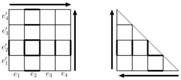
e1 e2 e3 e4 e0 1 e0 2 e0 3 e0 4
Figure 9: the construction of Ui; the bold lines represent U2
Note that (2) and (3) holds without orientability condition. Now we are ready to prove (3.1) (ii). For a map ρ : X→ |∆|, we define metric dρ on X by
(3.12) dρ(x, y) = d∆(ρ(x), ρ(y)) (x, y∈ X).
Proposition 3.16. Let ∆ be an orientable F-complex, and let Γ be its leg-graph. For
any map ρ : X→ |∆| on a finite set X, there exist maps ρi : X→ V Γ (i ∈ I) such that
dρ is a convex combination of dρi, and for any normal set R, ρ(x)∈ R implies ρ
i(x)∈ R
(i∈ I).
We may consider the case where ρ(X)⊆ V Γk for sufficiently large k. Each edge e of
Γ is subdivided into k edges e1, e2, . . . , ek. Fix an orientation of Γ with property (2.5).
Suppose that (e1, e2, . . . , ek) is arranged from the source to the sink in the orientation
of e. Let Ui be the set of edges projective to i-th edge ei. By construction, Ui∩ Uj =∅
for i6= j, and Ui is the union of orbits of ∆k; see Figure 9. By Proposition 3.15 (3), we
have dΓ(p, q) = 1 k k X i=1 d(Γk)Ui(pUi, qUi) (p, q∈ V Γ ).
Each ∆Ui is isomorphic to ∆ up to dilation factor 1/k. Therefore p 7→ pUi induces the
map φi:|∆| → V Γ . Then φi◦ρ (i = 1, 2, . . . , k) are desired maps. Also, by construction,
ρ(x)∈ σ implies ρi(x)∈ σ for any cell σ ∈ ∆. This implies the latter statement.
4
Related results
In this section, we present two results related to our argument. The first one is an optimal criterion of a combinatorial dual problem (2.7), which roughly characterizes the adjacency of extreme points of the feasible region in LP-dual (3.2). This result will play a crucial role in the splitting-off argument [13]. The second one is a characterization of distances of combinatorial dimension at most 2 in terms of F-complex realizations.
4.1 An optimality criterion for combinatorial dual problems
Here we show that (2.7) has an optimality criterion of the following type:
If ρ is not optimal, then there exists another ρ0 close to ρ having the smaller objective value.
We will characterize the closedness in terms of orientations of Γ . An orientation of
Γ with property (2.5) is said to be admissible. Admissible orientations are obtained
admissible. Each orbit has exactly two admissible orientations; one is the reverse of the
other one. A map ρ feasible to (2.7) is called a potential.
Let −→O be an oriented orbit by an admissible orientation. A potential ρ0 is called a
neighbor of a potential ρ with respect to−→O if for each x∈ V G with ρ0(x)6= ρ(x) (4.1) (i) there is an oriented edge −→pq∈−→O such that ρ(x) = p and ρ0(x) = q, or
(ii) there are two oriented edges −→pq, −→qr ∈−→O belonging to a common 2-cell in ∆
such that ρ(x) = p and ρ0(x) = r. Main theorem here is:
Theorem 4.1. If a potential ρ is not optimal, then there exists a neighbor ρ0 of ρ having the smaller objective value.
Remark 4.2. The combinatorial dual problem (2.7) is a variant of multifacility location
problem on graph Γ [24]. From the point of the view, Theorem 4.1 can be understood as
a generalization of a result of Dearing, Francis, and Lowe [5] for tree location problems (the case where Γ is a tree); see also [21, Chapter 3].
The proof is based on the idea used in [12]. A map ρ feasible to (2.6) is called a
continuous potential. We denote the distance among points ρ(x) by dρas (3.12), and also denote the corresponding objective valuePxy∈EGc(xy)dΓ(ρ(x), ρ(y)) simply byhc, dρi.
Recall the correspondence between metrics m feasible to (3.2) and a continuous po-tentials ρ, discussed in the beginning of Section 3. Namely, for a minimal feasible metric
m, there is a continuous potential ρ satisfying m = dρ. In general, this correspondence
m7→ ρ is not one-to-one. However one can establish the one-to-one correspondence by
the following trick. Add isolated terminals to S and extend µ so that{Rs}s∈S contains
all singleton sets of V Γ . In this case, the correspondence m 7→ ρ is one-to-one, and is continuous. Suppose that for a minimal feasible metric m there are two continuous potentials ρ, ρ0 with m = dρ = dρ0. Suppose ρ(x) 6= ρ0(x) for some x ∈ V G. Take minimal cells σ and σ0 of ∆ containing ρ(x) and ρ0(x), respectively. Suppose that σ and σ0 are distinct. Then there is a vertex v in σ such that d∆(v, ρ(x))6= d∆(v, ρ0(x)).
By the hypothesis, there is a terminal s with Rs = {v}. Then ρ(s) = ρ0(s) = v and
dρ(s, x) = dΓ(v, ρ(x)) 6= dΓ(v, ρ0(x)) = dρ
0
(s, x). A contradiction. Therefore σ = σ0. Since distances d∆(v, ρ(x))(= d∆(v, ρ0(x))) from vertices v of σ uniquely determines
ρ(x), two maps ρ and ρ0 must coincide.
We are ready to prove the statement. We remark that if the image of ρ belongs to V Γ , then dρ is minimal; this also follows from the fact that {Rs}s∈S contains all
singleton sets. Suppose that a potential ρ is not optimal. Equivalently, dρis not optimal to (3.2). Since dρis minimal and nonoptimal, there is another minimal feasible metric m0 sufficiently close to dρ such that hc, m0i < hc, dρi. By the minimality, m0 is represented by dρ0 for a continuous potential ρ0. Since m0 is sufficiently close to dρ and m0 7→ ρ0 is continuous, we may assume that
(4.2) d∆(ρ(x), ρ0(x)) < κ/2 (x∈ V G).
Recall that κ is the leg-length of ∆. Furthermore we may assume that ρ(V G)⊆ V Γk
for sufficiently large k. Fix some admissible orientation −→Γ of Γ . Decompose EΓk into
U1, U2, . . . , Uk and define maps φ1, φ2, . . . , φk : V Γ → V Γ as in the proof of
Proposi-tion 3.16. Then we have dρ0 = Pki=1dφi◦ρ0/k. Therefore there is an index i such that