Vol. 58, No. 2, April 2015, pp. 149–164
PROBABILISTIC ANALYSIS OF
LOAD-IMBALANCED PARALLEL APPLICATIONS WITH PARTIALLY ELIMINATED BARRIERS
Naoki Yonezawa Ken’ichi Katou Issei Kino Koichi Wada
Teikyo Heisei University Kanagawa University University of Tsukuba
(Received March 19, 2014; Revised August 22, 2014)
Abstract In order to reduce the overhead of barrier synchronization, we have proposed an algorithm which eliminates barrier synchronizations and evaluated its validity experimentally in our previous study. As a result, we have found that the algorithm is more effective to the load-imbalanced program than load-balanced program. However, the degree of the load balance has not been discussed quantitatively. In this paper, we model the behavior of parallel programs. In our model, the execution time of a phase contained in a parallel program is represented as a random variable. To investigate how the degree of the load balance influences the performance of our algorithm, we varied the coefficient of variation (CV) of probability distribution which the random variable follows. Using the model, we evaluated the execution time of parallel programs which have four typical dependency patterns. Based on results, we found that theoretical results are consistent with experimental ones.
Keywords: Information technologies, barrier elimination, probabilistic analysis, time
reduction
1. Introduction
Since barrier synchronization is a simple means to guarantee the order of data producing and data consuming, it is often used in parallel programs. However, barrier synchronization causes the processors’ idle time to increase. To reduce the overhead of barrier synchro-nization, several methods [1, 4, 7, 8] have been proposed. Tseng [4] proposed an algorithm to eliminate barrier synchronizations which appear SPMD (Single Program Multiple Data) program for shared memory multiprocessors and evaluate it on Stanford DASH [2]. He also proposed another algorithm to replace a barrier synchronization with a counter-based synchronization. The latter algorithm, in which consumers wait until a producer updates a variable, realizes synchronization among processors with smaller overhead than barrier synchronization. This method assumes the existence of a shared memory which DASH provides. Dwarkadas et al. [1] proposed a method for their compiler to replace a barrier synchronization with push function in which producer sends updated data to consumers.
In our method [7, 8] which targets on the distributed shared memory environment realized on a PC cluster, the compiler analyzes the dependency between the data producers and the data consumers. Then, the compiler replaces the barrier synchronization with message passing code which sends the data to consumer’s side. Through evaluation, we have found that the algorithm is more effective to the load-imbalanced program than load-balanced program. However, the degree of the load balance has not been discussed quantitatively.
In this paper, in order to analyze the effect of the method theoretically, we propose a probabilistic model to describe the degree of the load balance and evaluate the effectiveness
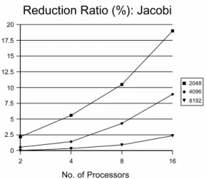
Figure 1: The ratio of improvement: Jacobi method
Figure 2: The ratio of improvement: Gauss method
of a barrier eliminating algorithm in terms of the load balance. In above two methods [1, 4], however, some theoretical model is not constructed and no mathematical evaluation is carried out. Sun and Peterson [3] represent the execution time by using random variables as in this paper. However, they focus on a method to approximate the execution time while we aim to optimize parallel programs by eliminating barriers partially.
The rest of this paper is organized as follows: Section 2 describes the algorithm to eliminate barriers on which our study targets. In Section 3, we propose a probabilistic model to investigate the barrier eliminating algorithm. With the model, one can describe data dependencies among processors as well as the degree of the load balance. We also show how to compute the execution time of a parallel program mathematically. Using the results obtained from our model, Section 4 discusses the effect of the barrier eliminating algorithm when applied to four typical dependency patterns. Finally, we conclude our study and describe our future work in Section 5.
2. A Barrier Eliminating Algorithm
A compiler which uses the barrier eliminating algorithm replaces barrier synchronizations with send-receive pairs as follows: 1) the compiler identifies accesses to the shared memory
Figure 3: Eliminating barriers
and represents the accesses using array section descriptor called quad [6], 2) to investigate a dependency between data producer and data consumer, the compiler generates an intersec-tion operaintersec-tion between quads which represent write accesses which are performed before the barrier and read accesses which are performed after the barrier, 3) the compiler generates a send-receive pair to transfer the dependent data which are represented by the resulting quad yielded by the intersection operation and eliminates the barrier.
In the former study [7, 8], the effect of the barrier eliminating algorithm is investigated experimentally. Figure 1 shows the ratio of improvement which is computed as 100× (1 − Ta/Tb), where Tb is the execution time of Jacobi method before eliminating barriers and Tais
the one after eliminating barriers. Figure 2 shows the results for Gauss method. The size of matrix is varied from 2,048 to 8,192. These applications are executed on a PC cluster which consists of Gigabit Ethernet and 16 PCs, each of which has Intel Xeon 2.8 GHz and 1 GB memory. It is observed that the ratio increases as the number of processors grows. We also have found that the barrier eliminating algorithm is more effective on the load-imbalanced program, i.e., Gauss method than Jacobi method.
3. A Probabilistic Analysis of a Barrier Eliminating Algorithm
In this section, at first, we define a behavioral model of a parallel program and introduce the mathematical symbols for discussion. Then, we construct the probabilistic model which describes the behavior of parallel program. Finally, we compute the effect of barrier elimi-nation mathematically using the simplest example in which both the number of processors and the number of phases are two.
3.1. The behavioral model of parallel program 3.1.1. Before eliminating barriers
Figure 3 (a) shows the behavioral model of a parallel program on which this paper targets. In this model, a program contains a loop whose iteration has one and only barrier syn-chronization. We call an iteration of the loop a phase. The task in a phase is divided into n subtasks and the subtasks are assigned to n processors. At runtime, when a processor arrives a barrier synchronization, the processor stalls. After all the other processors arrives the barrier synchronization, all processors execute the next phases.
It is expected that the execution times of a phase are equal among processors if the phase contains the equally-divided subtasks and a barrier synchronization. However, the execution of a parallel program in the real world is influenced by the external factors including cache misses and the network delay. These cause randomness, i.e., the execution time of a processor in a phase can differ from the one of another processor in the same phase. In order to model the execution of such programs, we denote the execution time of Processor j in Phase i by Xj(i), i = 1, 2, . . . , j = 1, 2, . . . , n, where {{Xj(i)}n
j=1}∞i=1 are independent and identically
distributed random variables (i.i.d. r.v.’s). At this time, the execution time of Phase i is Tn(i) = max(X1(i), X2(i), . . . , Xn(i)) because the execution time of the phase is the execution
time of the slowest processor. Therefore, the execution time of m phases with n processors before eliminating barriers is Bn(m) = Tn(1)+ Tn(2)+· · · + Tn(m) and the mean execution time
becomes E(Bn(m)) = mE(Tn(1)).
3.1.2. After eliminating barriers partially
In this paper, we use the term dependent on part to represent a situation that a processor depends on several processors rather than all other processors. Dependent on part situations appear in many parallel programs. On the other hand, the term dependent on all represents a situation that a processor depends on all other processors. The case of ‘before eliminating barriers’ we showed in Section 3.1.1 is dependent on all throughout all phases.
Figure 3 (b) shows an example of the behavioral model of a parallel program after eliminating barrier partially. For instance, at the beginning of Phase 2, Processor 1 has to wait for the finish of Phase 1 performed by Processor 2 while Processor 3 and 4 do not need to wait for Processor 2 and can proceed Phase 2 asynchronously. In this example, Processor 1 does not stall because the necessary data have arrived at Processor 1 from Processor 2 before the beginning of the Phase 2. At the beginning of Phase 3, Processor 2 has to wait for the finish of Phase 2 performed by Processor 3 and 4. In this example, while the finish of Phase 2 performed by Processor 3 precedes the finish of Phase 2 performed by Processor 2, the finish of Phase 2 performed by Processor 4 is behind with the finish of Phase 2 performed by Processor 2. This delay makes Processor 2 idle.
In general, before Processor j proceeds Phase i in dependent on all situation, it has to wait for the finish of Phase (i− 1) performed by all other processors. On the other hand, in dependent on part situation, Processor j has to wait for the finish of Phase (i−1) performed by not all but several processors as shown in Figure 3 (b). In this paper, we call depended processors of Processor j in Phase i a group of the processors for which Processor j has to wait at the beginning of Phase i. We denote by Sj(i) the set of depended processors’ IDs. Note that about Sj(i):
• j ∈ S(i)
j because Processor j always depends on itself.
• S(1)
j is empty set for all j because there is no memory access before Phase 1.
program, that is Phase 1, to the end of Phase i. Xj(1,i) is decomposed as follows: Xj(1,i) = max ( Xk(1,i−1) ) k∈S(i)j + Xj(i), i = 2, 3, 4, . . .
In other words, Xj(1,i) is the sum of the longest execution time of depended processors at the end of Phase (i− 1) and the execution time of Phase i performed by Processor j.
We also denote the execution time of the program in which all processors execute by A(m)n .
Then, A(m)n = max(X1(1,m), X (1,m)
2 , . . . , X (1,m)
n ), that is, the random variable A(m)n represents
the execution time of m phases with n processors after eliminating barriers partially.
3.2. The definition of dependency matrix
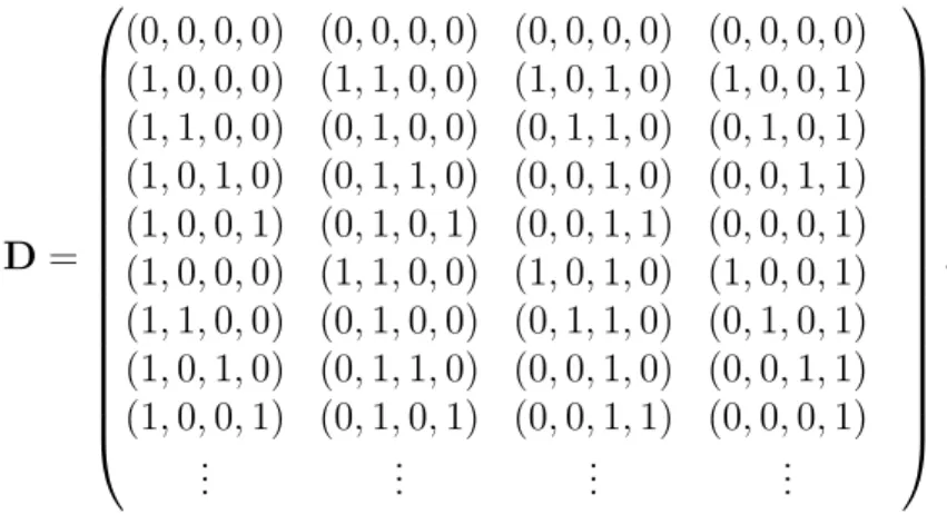
To represent partial dependency, it is necessary to describe depended processors, that is, the group of processors for which a processor has to wait at the beginning of a phase. To achieve this, we propose a dependency matrix in this paper as follows:
D = d11 d12 . . . d1n d21 d22 . . . d2n .. . ... . .. ... dm1 dm2 . . . dmn .
The element of matrix D is a binary vector dij. The size of dij is equal to the number of
processors, that is, |dij| = n. Each element of dij represents dependency among processors.
More specifically,
k-th element of dij =
{
1, if k ∈ Sj(i) 0, if k /∈ Sj(i).
If k-th element of dij is 1, Processor j has to wait for Processor k at the beginning of Phase
i.
The following is an example of dij:
d35 = (0, 1, 0, 0, 1, 1).
In this example, the number of processors is 6 due to|d35| = 6. d35represents that Processor
5 has to wait the end of Phase 2 performed by Processor 2, 5, and 6 at the beginning of Phase 3. Because Processor 5 has to wait for itself, the fifth element of di5, i = 1, 2, . . . , m
is always 1.
3.3. Obtaining a function to calculate the execution time
The overall execution time is determined by the execution time of each phase, that is X1(1), . . . , Xn(m). Therefore, we denote the overall execution time by a function T (X1(1), . . . , X
(m)
n ).
The specific form of the function T (X1(1), . . . , Xn(m)) is depended on the content of
depen-dency matrix D. In general, T is constructed from multistage and nested operations of max(·) and addition. The following algorithm constructs T recursively starting from the last phase.
Algorithm 1:
Input: dependency matrix D, the number of phases m, the number of processors n.
Output: a function A(m)n = T (X1(1), . . . , X (m)
n ) to calculate the execution time with mn
random variables as parameters. 1. i← m.
2. Obtain An(i) = max(X(i)), where X(i) = (X1(1,i), X2(1,i), ..., Xn(1,i)).
3. Substitute Xj(1,i) with max(dij ∧ X(i−1)) + X
(i)
j , where ∧ is an operator which return a
list whose element is a product of the corresponding elements of two lists of operands. 4. i← i − 1.
5. If i is 1 then go to the end, otherwise go to Step 3.
3.4. Probability distribution of the execution time
The performance of barrier elimination may vary significantly depending on the distribution of random variables which represent the execution time for each processor and each phase. In this study, we assume that a random variable follows one of three distributions: exponential distribution, Erlang distribution, and hyper-exponential distribution.
In exponential distribution whose parameter is λ, the CDF for Xj(i) is assumed in the form
F (x) = P (Xj(i) ≤ x) = 1 − e−λx
for i = 1, 2, . . . and j = 1, 2, . . . , n, so that the PDF is in the form f (x) = λe−λx and expected value (mean execution time) becomes E(Xj(i)) = λ1.
The CDF and the PDF of Erlang distribution are
F (x) = 1− e−λkx k−1 ∑ r=0 (λkx)r r! , (3.1) f (x) = (λk) k (k− 1)!x k−1 e−λkx, (3.2)
where k is the number of phases∗. The expected value of random variables which follow the above Erlang distribution is also 1
λ.
The CDF and the PDF of hyper-exponential distribution are
F (x) = 1− k ∑ j=1 Cje−λjx, f (x) = k ∑ j=1 Cjλje−λjx,
where {Cj}kj=1 is an arbitrary discrete distribution. As mentioned later, we will choose
parameters Cj and λj so that E(X
(i)
j ) =
1
λ.
The adoption of these distributions for the execution time is based on the following idea. For non-negative random variables with the same expected value, the coefficient of variation (CV) is the most useful and popular characteristic parameter for comparing the degree of variation. The CV c(X) for non-negative random variable X is defined by
c(X) = √
V (X) E(X)
where V (X) is variance of X, i.e., V (X) = E(X2) − E(X)2. It is clear that for fixed
value of E(X), as increases the value of c(X), the variance of X also increases. In the field
∗The term of phase which is used in the context of probability theory is unrelated to a phase which is included in parallel program.
of probability theory, exponential distribution, Erlang distribution, and hyper-exponential distribution are the most typical distribution with different CV. It is well known that c(X) = 1 for exponential distribution, c(X) < 1 for Erlang distribution, and c(X) > 1 for hyper-exponential distribution. In other words, for the same expected value, Erlang distribution shows lower variance and hyper-exponential distribution shows higher variance comparing with exponential distribution.
One can use, therefore, c(X) as an impact factor of difference of distribution to the performance of barrier elimination. For example, Jacobi method which is a typical load-balanced program should be modeled with Erlang distribution whose c(X) < 1, whereas it is reasonable to consider that Gauss method corresponds to c(X) > 1.
3.5. An example: the case of m = 2, n = 2
A dependency matrix can represent various kinds of dependency patterns among processors including the case in which all barriers are eliminated and the case in which all barriers are remained.
In this section, we construct three functions in the simplest case of m = 2, n = 2 using three kinds of dependency matrices. Hereafter, we denote by B2(2), A∗(2)2 , and A(2)2 the execution time of the case in which all barriers are remained, all barriers are eliminated, and a single barrier is eliminated respectively.
3.5.1. Case 1: remaining all barriers
The dependency matrix in the case that all barriers are remained is
D = ( (0, 0) (0, 0) (1, 1) (1, 1) ) . The function of the execution time is
B2(2) = max(X(2)) = max(X1(1,2), X2(1,2)), X1(1,2) = max(d21∧ X(1)) + X (2) 1 = max((1, 1)∧ (X1(1,1), X2(1,1)) + X1(2) = max(X1(1,1), X2(1,1)) + X1(2) = max(X1(1), X2(1)) + X1(2), X2(1,2) = max(d22∧ X(1)) + X2(2) = max((1, 1)∧ (X1(1,1), X2(1,1)) + X2(2) = max(X1(1,1), X2(1,1)) + X2(2) = max(X1(1), X2(1)) + X2(2). 3.5.2. Case 2: eliminating all barriers
The dependency matrix in the case that all barriers are eliminated is
D = ( (0, 0) (0, 0) (1, 0) (0, 1) ) . The function of the execution time is
X1(1,2) = max(d21∧ X(1)) + X (2) 1 = max((1, 0)∧ (X1(1,1), X2(1,1)) + X1(2) = max(X1(1,1), 0) + X1(2) = X1(1)+ X1(2), X2(1,2) = max(d22∧ X(1)) + X (2) 2 = max((0, 1)∧ (X1(1,1), X2(1,1)) + X2(2) = max(0, X2(1,1)) + X2(2) = X2(1)+ X2(2). 3.5.3. Case 3: eliminating a single barrier
We assume that Processor 1 waits for itself at the beginning of Phase 2 while Processor 2 waits for both processors. The dependency matrix in this case is
D = ( (0, 0) (0, 0) (1, 0) (1, 1) ) . The function of the execution time is
A(2)2 = max(X(2)) = max(X1(1,2), X2(1,2)), X1(1,2) = max(d21∧ X(1)) + X1(2) = max((1, 0)∧ (X1(1,1), X2(1,1)) + X1(2) = max(X1(1,1), 0) + X1(2) = X1(1)+ X1(2), X2(1,2) = max(d22∧ X(1)) + X (2) 2 = max((1, 1)∧ (X1(1,1), X2(1,1)) + X2(2) = max(X1(1,1), X2(1,1)) + X2(2) = max(X1(1), X2(1)) + X2(2). 4. Evaluation
To investigate how much impacts brought by the differences of the load balance among processors in executing parallel programs on the effect of the barrier eliminating algorithm, we calculated the execution time for four kinds of dependency patterns (DPs) with varying the coefficient of variation.
We calculated the execution time using Monte Carlo simulation as shown in Algorithm 2. We varied the number of phases m = {2, 3, . . . , 10} as well as the number of processors n = {2, 4, 8, 16, 32}. We made four kinds of typical dependency patterns and stored them in dependency matrices D. The details of each D are described later.
In this evaluation, as mentioned in Section 3.4, we assume that all random variables Xj(i) follow exponential distribution, Erlang distribution, or hyper-exponential distribution.
Table 1: Coefficients of variation (CV)
E100 E4 E2 M H2
0.1000 0.5000 0.7071 1.0000 1.5100
We chose parameters of hyper-exponential distribution so that all of their expected value is equal to 1λ as in two other distributions. As a result, we obtained the PDF of hyper-exponential distribution as follows:
f (x) = 5 2λe −5λx+ 5 18λe −5 9λx.
We also chose parameter k for Erlang distribution, which appears in Equation (3.1) and (3.2), as k ={2, 4, 100}. We denote exponential distribution, Erlang distribution with parameter k, and hyper-exponential distribution by M, Ek, H2, respectively, derived from
Kendall’s notation in queuing theory.
Table 1 shows CVs for the five distributions.
Hereafter, we assume that λ = 1 without loss of generality.
Algorithm 2:
Input: the number of steps N , dependency matrix D, the number of phases m, the number of processors n.
Output: the execution time.
1. As described in Section 3.3, obtain a function T (X1(1), . . . , Xn(m)) with mn random
vari-ables as parameters based on D. 2. i← 1.
3. S ← 0.
4. Assign random numbers which follow a probability distribution to mn random variables. 5. S ← S + T (X1(1), . . . , Xn(m)).
6. i← i + 1.
7. If i is N + 1 then go to Step 8, otherwise go to Step 4. 8. Output NS.
We performed five simulations for a pair of (m, n) with the initial number of steps N , that is, 103. We consider that the simulations are successful if all the five execution times are equal when the times are rounded off to the second decimal place. If the rounded times are not equal, we increase N by ten, and then perform five simulations again. Consequently, we observed that 45 simulations for all pairs of (m, n) are successful before N reached 1010.
4.1. Dependency Pattern 1: depending on the neighboring processors
In DP-1, a processor depends on neighbors and itself. More exactly, Processor j depends on Processor j− 1, j, and j + 1. Exceptionally, Processor 1 depends on Processor 1 and 2 as well as Processor n depends on Processor n− 1 and n. This dependency pattern appears in some applications including image processing and physics simulation, in which the value of a point is computed using neighboring points. The part of D for n = 4 used in DP-1 is as follows: D = (0, 0, 0, 0) (0, 0, 0, 0) (0, 0, 0, 0) (0, 0, 0, 0) (1, 1, 0, 0) (1, 1, 1, 0) (0, 1, 1, 1) (0, 0, 1, 1) (1, 1, 0, 0) (1, 1, 1, 0) (0, 1, 1, 1) (0, 0, 1, 1) .. . ... ... ... .
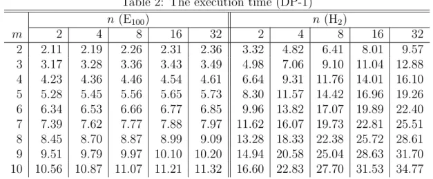
Table 2: The execution time (DP-1) n (E100) n (H2) m 2 4 8 16 32 2 4 8 16 32 2 2.11 2.19 2.26 2.31 2.36 3.32 4.82 6.41 8.01 9.57 3 3.17 3.28 3.36 3.43 3.49 4.98 7.06 9.10 11.04 12.88 4 4.23 4.36 4.46 4.54 4.61 6.64 9.31 11.76 14.01 16.10 5 5.28 5.45 5.56 5.65 5.73 8.30 11.57 14.42 16.96 19.26 6 6.34 6.53 6.66 6.77 6.85 9.96 13.82 17.07 19.89 22.40 7 7.39 7.62 7.77 7.88 7.97 11.62 16.07 19.73 22.81 25.51 8 8.45 8.70 8.87 8.99 9.09 13.28 18.33 22.38 25.72 28.61 9 9.51 9.79 9.97 10.10 10.20 14.94 20.58 25.04 28.63 31.70 10 10.56 10.87 11.07 11.21 11.32 16.60 22.83 27.70 31.53 34.77
Dependency is fixed as phase ID increases.
Table 2 shows the execution time for E100 and H2. To avoid redundancy, the results for
three other distributions are not shown but their values take place between E100 and H2.
As mentioned above, the expected value of the execution time for a single phase is 1 (=λ1). For n = 2, the dependency pattern is identical to the pattern in the case that all barriers are remained. Furthermore, with respect to E2, M, and H2, the execution time obtained by
simulation for n = 2 is identical to the execution time obtained by mathematical analysis shown in Yonezawa et al. [5], in which it is assumed that a random variable follows one of E2, M, and H2. Therefore, this imply the correctness of our simulation.
4.2. Dependency Pattern 2: depending on a single specific producer
In DP-2, all processors depend on a single specific producer. It is also known as ‘single writer, multiple reader’. This pattern appears in master-worker type applications. The part of D for n = 4 used in DP-2 is as follows:
D = (0, 0, 0, 0) (0, 0, 0, 0) (0, 0, 0, 0) (0, 0, 0, 0) (1, 0, 0, 0) (1, 1, 0, 0) (1, 0, 1, 0) (1, 0, 0, 1) (1, 0, 0, 0) (1, 1, 0, 0) (1, 0, 1, 0) (1, 0, 0, 1) .. . ... ... ... .
As in DP-1, dependency is fixed as phase ID increases. Table 3 shows the execution time.
4.3. Dependency Pattern 3: depending on rotating producers
DP-3 is similar to DP-2 since all processors depend on a single producer. However, pro-ducer’s ID is incremented when processors go to the next phase in DP-3. If Processor n is the producer in a phase, Processor 1 becomes the next producer in the next phase. This pattern appears in some applications including Gaussian elimination method in which the rows of matrix is assigned to processors in block-cyclic manner. The part of D for n = 4
Table 3: The execution time (DP-2) n (E100) n (H2) m 2 4 8 16 32 2 4 8 16 32 2 2.10 2.17 2.23 2.28 2.32 3.19 4.56 6.01 7.45 8.87 3 3.13 3.22 3.29 3.35 3.40 4.64 6.35 8.03 9.64 11.20 4 4.16 4.26 4.34 4.41 4.47 6.04 8.02 9.88 11.63 13.31 5 5.18 5.30 5.39 5.47 5.53 7.40 9.61 11.63 13.50 15.27 6 6.21 6.34 6.43 6.52 6.59 8.74 11.15 13.30 15.28 17.14 7 7.23 7.37 7.47 7.56 7.64 10.05 12.64 14.92 16.99 18.93 8 8.25 8.40 8.51 8.60 8.68 11.34 14.10 16.49 18.65 20.67 9 9.27 9.43 9.54 9.64 9.73 12.62 15.53 18.03 20.27 22.36 10 10.28 10.45 10.58 10.68 10.77 13.88 16.94 19.53 21.85 24.01
Table 4: The execution time (DP-3)
n (E100) n (H2) m 2 4 8 16 32 2 4 8 16 32 2 2.10 2.17 2.23 2.28 2.32 3.19 4.56 6.01 7.45 8.87 3 3.14 3.23 3.30 3.36 3.41 4.74 6.51 8.21 9.83 11.40 4 4.18 4.30 4.37 4.44 4.50 6.30 8.46 10.38 12.14 13.80 5 5.23 5.36 5.45 5.52 5.58 7.85 10.46 12.54 14.42 16.16 6 6.27 6.43 6.52 6.59 6.66 9.40 12.44 14.72 16.68 18.48 7 7.31 7.49 7.59 7.67 7.73 10.95 14.42 16.90 18.93 20.78 8 8.36 8.56 8.67 8.74 8.81 12.50 16.41 19.10 21.18 23.08 9 9.40 9.62 9.74 9.82 9.89 14.05 18.39 21.30 23.43 25.36 10 10.44 10.69 10.81 10.89 10.96 15.60 20.37 23.50 25.69 27.64 used in DP-3 is as follows: D = (0, 0, 0, 0) (0, 0, 0, 0) (0, 0, 0, 0) (0, 0, 0, 0) (1, 0, 0, 0) (1, 1, 0, 0) (1, 0, 1, 0) (1, 0, 0, 1) (1, 1, 0, 0) (0, 1, 0, 0) (0, 1, 1, 0) (0, 1, 0, 1) (1, 0, 1, 0) (0, 1, 1, 0) (0, 0, 1, 0) (0, 0, 1, 1) (1, 0, 0, 1) (0, 1, 0, 1) (0, 0, 1, 1) (0, 0, 0, 1) (1, 0, 0, 0) (1, 1, 0, 0) (1, 0, 1, 0) (1, 0, 0, 1) (1, 1, 0, 0) (0, 1, 0, 0) (0, 1, 1, 0) (0, 1, 0, 1) (1, 0, 1, 0) (0, 1, 1, 0) (0, 0, 1, 0) (0, 0, 1, 1) (1, 0, 0, 1) (0, 1, 0, 1) (0, 0, 1, 1) (0, 0, 0, 1) .. . ... ... ... .
Unlike DP-1 and 2, dependency is varied as phase ID increases.
Table 4 shows the execution time. For m = 2, because dependency pattern is identical to the pattern in DP-2, the execution time in DP-3 is also identical to the execution time in DP-2.
Table 5: The execution time (DP-4) n (E100) n (H2) m 2 4 8 16 32 2 4 8 16 32 2 2.11 2.18 2.24 2.29 2.34 3.32 4.69 6.17 7.67 9.16 3 3.17 3.26 3.33 3.39 3.45 4.98 6.86 8.65 10.42 12.14 4 4.23 4.33 4.42 4.49 4.56 6.64 9.02 11.17 13.17 15.08 5 5.28 5.41 5.51 5.59 5.66 8.30 11.19 13.69 15.94 18.03 6 6.34 6.49 6.59 6.68 6.76 9.96 13.35 16.21 18.71 20.98 7 7.39 7.56 7.68 7.78 7.86 11.62 15.52 18.72 21.48 23.94 8 8.45 8.64 8.77 8.88 8.97 13.28 17.68 21.24 24.25 26.89 9 9.51 9.71 9.86 9.97 10.07 14.94 19.85 23.76 27.01 29.85 10 10.56 10.79 10.95 11.07 11.17 16.60 22.01 26.27 29.78 32.80
Figure 4: The ratio of improvement (m = 10; n = 8)
4.4. Dependency Pattern 4: butterfly operation
DP-4 represents butterfly operation which appears in fast Fourier transform (FFT). The part of D for n = 4 used in DP-4 is as follows:
D = (0, 0, 0, 0) (0, 0, 0, 0) (0, 0, 0, 0) (0, 0, 0, 0) (1, 1, 0, 0) (1, 1, 0, 0) (0, 0, 1, 1) (0, 0, 1, 1) (1, 0, 1, 0) (0, 1, 0, 1) (1, 0, 1, 0) (0, 1, 0, 1) (1, 1, 0, 0) (1, 1, 0, 0) (0, 0, 1, 1) (0, 0, 1, 1) (1, 0, 1, 0) (0, 1, 0, 1) (1, 0, 1, 0) (0, 1, 0, 1) .. . ... ... ... .
As in DP-3, dependency is varied as phase ID increases. Table 5 shows the execution time.
4.5. Discussion
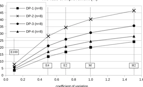
Figure 4 and Figure 5 shows the ratio of improvement which is calculated by 100×(1−Tp/Tb),
Figure 5: The ratio of improvement (m = 10; n = 32)
execution time in DP-1, -2, -3, or -4 for m = 10 and n = 8, 32.
The common trends among four kinds of DPs are 1) if CV increases, namely, if the loads among processors is more imbalanced, the ratio of improvement also increases, 2) if n, the number of processors, increases, the ratio of improvement also increases. These trends are also observed in Yonezawa et al. [5]. For example, the ratio of improvement in the case that all random variables follow E100 is 11.87% for n = 32 in DP-2 while the ratio in the
case that all random variables follow H2 is 60.37%. Since the program contains much idle
time for H2, once barriers are partially eliminated, the opportunities to move the execution
of phases forward increases. This decreases idle time and therefore increases the ratio of improvement. If n increases, the deviation of the execution time among processors increases. This causes idle time if all barriers are remained. Eliminating several barriers mitigates the deterioration for larger n.
The ratio of improvement in DP-2, -3, and -4 are greater than DP-1. It is caused by the number of depended processors. In general, when the number of 1s included in dependency matrix D increases, the number of depended processors also increases. In this evaluation, the number of 1s in D for DP-2 is equal to the one for DP-3 while D for DP-4 has more 1s than these DPs and D for DP-1 has the most 1s.
Whereas the number of 1s in D is the same between DP-2 and -3, the execution times differ. In DP-3, a producer in a phase depends on the previous producer directly. However, there are depended producers which influence indirectly from the past phases. This makes a chain of dependency across phases and the producer in Phase j, j > n, depends on all processors directly or indirectly.
DP-1 spends more time compared with three other DPs. It is caused by the number of chains of dependency. In DP-1, a processor depends on two neighbors. Therefore, two chains are generated for the processor. This brings rapid growth of the number of depended processors indirectly.
In this paper, we consider an imaginary optimal situation, where all barriers are re-moved and all phases are performed consecutively with disregarding dependencies among processors. Consequently, the execution time include no idle time in the situation and is
Figure 6: Optimal degree (DP-1: n = 32)
regarded as the upper bound of the effect of barrier eliminating method. We call the relative execution time optimal degree, which are calculated based on the optimal execution time. Although the value of optimal degree can be affected by the kinds of DPs and CVs, in order to avoid redundancy, we show the result with varying CV while fixing DP. One can consider that a CV is near to optimal if the optimal degree is close to 1. Figure 6 shows optimal degree for n = 32 in DP-1. While we omit the results for three other DPs, optimal degree tends to decrease when CV increases in four DPs. For example, optimal degree in the case that all random variables follow E100 is 0.94 with m = 10 while optimal degree in the case
that all random variables follow H2 is 0.64. With E100, the idle time are inherently short
even if all barriers are remained due to a good load balance. In contrast to E100, H2 causes
long idle time, which cannot be removed even after several barriers are eliminated.
Figure 7 shows speedup for m = 10 in DP-1, which is calculated based on mn(= mnλ ), that is, the execution time for uniprocessor. Speedup tends to decrease when CV increases. For example, the maximum speedup is 28.27 for n = 32 when all random variables follow E100. In contrast, the speedup is limited to 9.20 for H2.
Throughout evaluation, we found that the obtained effect of eliminating barriers is higher if a processors depends on less other processors. Even if a processor depends on few other processors, the excess barriers force the processor to wait for other non-depended processors. If a processor depends on quite a few other processors as in DP-3, the effect of eliminating barriers is limited due to the necessary interprocessor communications even after eliminating barriers. With regard to the load balance, we found that a better speedup is obtained if a load balance is better while the less effect of eliminating barrier is obtained. If loads among processors are imbalanced as in H2, barrier elimination can contribute to improve
the performance of parallel programs. These observations are consistent to the experimental results we have shown in Figure 1 and 2.
5. Conclusion
In this paper, we proposed a probabilistic model which describes the behavior of a parallel program and measured the effect of the algorithm of barrier elimination. In our model, random variables show the execution time for one phase in which one processor performs. By introducing dependency matrix, we extended the model we have proposed in our previous
Figure 7: Speedup (DP-1: m = 10)
work so that our extended model represents dependencies among processors.
For evaluation, we executed four kinds of parallel program in simulation. In order to investigate how a load balance influences the effect of barrier eliminating method, we adopted three probability distributions, that is, exponential distribution, Erlang distribution, and hyper-exponential distribution. We obtained the ratio of improvement, the optimal degree, and the speedup. Based on these results, we found that a better speedup is obtained if a load balance is better while the less effect of eliminating barrier is obtained.
In the future, we plan to extend our study as follows:
• we will make our study more accurate by sampling execution times of processors at runtime of real applications and then applying the samples to our model.
• we will extend dependency matrix to represent dependencies with respect to not only a previous phase but also two or more previous phases.
• we will evaluate other typical dependency patterns such as a reduction operation. • the structure of dependency matrix which is proposed in this paper is too complex to
apply algebraic operations. In the future, we will propose several simple dependency matrices and primitive operations among them. By combining such matrices as building blocks, we construct desired dependency matrices which represent more complicated dependency patterns. We might find a correlation between the constructing process of a dependency matrix and the execution time which is derived from the matrix.
References
[1] S. Dwarkadas, A. L. Cox and W. Zwaenepoel: An Integrated Compile-Time/Run-Time Software Distributed Shared Memory System. In Proceedings of International Con-ference on Architectural Support for Programming Languages and Operating Systems (1996), 186–197.
[2] D. Lenoski, J. Laudon, K. Gharachorloo, W.-D. Weber, A. Gupta, J. Hennessy, M. Horowitz and M. S. Lam: The Stanford DASH Multiprocessor. Computer, 25 (1992), 63–79.
[3] J. Sun and G.D. Peterson: An Effective Execution Time Approximation Method for Parallel Computing. IEEE Trans. Parallel Distrib. Syst., 23 (2012), 2024–2032.
[4] C.-W. Tseng: Compiler Optimizations for Eliminating Barrier Synchronization. In Pro-ceedings of the Fifth ACM SIGPLAN Symposium on Principles and Practice of Parallel Programming (1995), 144–155.
[5] N. Yonezawa, I. Kino and K. Wada: Probabilistic analysis of time reduction by eliminat-ing barriers in parallel programmes. International Journal of Communication Networks and Distributed Systems, 6 (2011), 404–419.
[6] N. Yonezawa and K. Wada: quad : Array Section Descriptor for Parallel Computing. IPSJ Journal, 46 (2005), 1274–1286 (in Japanese).
[7] N. Yonezawa and K. Wada: Reducing Idle Times on Matrix Programs by Eliminating Barrier Synchronization. IEICE Journal, J91-D (2008), 907–921 (in Japanese). [8] N. Yonezawa, K. Wada and T. Aida: Barrier Elimination Based on Access
Depen-dency Analysis for OpenMP. In Proceedings of International Symposium on Parallel and Distributed Processing and Applications (2006), 362–373.
Naoki Yonezawa
Department of Business Management Teikyo Heisei University
4-21-2 Nakano, Nakano Tokyo 164-8530, Japan