AN ALGORITHM FOR A MULTIOBJECTIVE, MULTILEVEL LINEAR PROGRAMMING

Journal of t.he 0perat.ions Research Society of Japan

Vol. 39, No. 2, June 1996

AN ALGORITHM FOR A MULTIOBJECTIVE,

MULTILEVEL LINEAR PROGRAMMING

Zhi- Wei Wang Hiroyuki Nagasawa Noriyuki Nishiyama Shinwa Kogyo C o . Osaka Prefecture University Osaka Institute of Technology

(Received May 30, 1994; Final January 26, 1996)

Abstract This paper discusses a solut,ion method to a multiobjective, multi-level decentralized system. A decomposition method is proposed for dividing the n-level problem finally into n

-

2 single level problems a,nd a two-level problem. A method with dominattion trees based on the "two-level simplex algorithm" is developed for generating the nondominated solutions to this type of n-level decentralized system.

1. I n t r o d u c t i o n

In a multi-level decentralized system consisting of one hea.clquarters, several divisions and

factories

[2]

,

it is required t o make its decision considering not only a competition with others

but also the coexistence with the social environment t o pursuit the overall development of the corporation.

From the strategic view points, the headquarters is forced in such a circumstance to con- sider the second and third objectives in making its decision, while the objectives of divisions and fa,ctories remain single. This type of decentralized system is called a "multiobjective, multilevel decentralized system" in this paper.

A

multi-level decentralized linear system can generally be represented as a multi-level

linear programming problem [l]

,

but so far there is no solution method proposed for dealing

with a multiobjective, multilevel decentralized system.

This pa.per first formulates a mathematical model for a multiobjective, multilevel de-

centralized system.

A

method for generating all the nondominated solutions to this model

is proposed and a numerical example of a two-objective, there-level decentralized system is demonstraied to show the effectiveness of the proposed method.

2.

M o d e l F o r m u l a t i o n

A

corporation adopting a decentralized decision-making system can be described as a

multi-level decentralized system as shown in Fig. 1. T h e first (top) level in Fig. 1 means the headquarters of the c ~ r p o r a ~ t i o n and the second level, various divisions. The headquarters allocates gross resources such as budget, man power, energy, raw materials and facilities among the divisions. Ea,ch division makes a.n aggregate production plan and resource allo- cation for factories belonging to the division. Factories located a t the third level shown in Fig. 1 produce different types of products, using the resources allocated by their divisions.

In general, a multiobjective, n-level decentralized system described above is mathemat- ically formulated in the following a,ggregated form:

[ P r o b l e m

P(")]

<

t h e 1 s t l e v e l p r o b l e m

>

Algorithm for Multiobjective, Multilevel LP

1

Headquarters

-1

T h e 1st division

...

T h e

(1,l)

factory

factory

1

T h e Icth division

1

I r

T h e

(I<,l)

T h e

(I<,

nI<) a . .

factory

factory

I

Fig.1 Organization of

a

three-level decentralized system

(---

--

Flow of resource allocation plan.

-

Flow of production plan)

subject to

Glyl

S

Y l ,

Y l

2

0,

<

the

2nd

level problem

>

Maximize

f 2 ( ~ 2 ) = { c 2 x ( y n , - l ( . ( ~ 3 ( ~ 2 ) ) ) ) - c n , - 1 , 2 y n - l ( ~ n - 2 ( - ( y 3 ( y 2 ) ) ) ) - ~ n - 2 , 2 y n - 2 ( ~ n - 3 ( -

.

( ~ 3 ( ~ 2 ) ) ) ) - - ~ 3 , 2 ~ 3 ( ~ 2 ) } - C 2 , 2 y 2 , subject to

G2y2

Y2

+

Dsyl,

y 2

2

0,

<

the ( n -

1 ) t h

level problem

>

Maximize fn(x) = cnx,

subject to

_AX

=

b

+

Dnyn-l)

X

2

0,

where the notations a,re defined below.

L:

number of objective functions of the headquarters

X: production amount vector to be planned a t the n t h level (including slack variables

if

these

178 2.- W. Wang, H, Nagasawa & N. Nishiyama

x(yn-1): optimal solution to the n t h level problem with the resource given by yn-1

y i { ~ i - ~ ) : optima,l solution to the i-level problem with the resource given by yi-1, i =

2,3,

...,

n - 1

x(yn-l(.

. .

(yi+l ( y j ) ) ) ) : information on the optimal production amount determined at the n t h level, fed back to the j t h level

yi(yi-l(.

.

( ~ j + ~ ( y ~ ) ) ) ) : information on the optimal resource allocation determined a t the it11 level, fed back to the j t h level, i = j

+

l ,

.,.

.

, n -

1,

j = 1 , 2 , .

. .

, n - 2

D,:

constraint ma,trix with respect t o the resource yi-1 allocated from the (i - 1)th level t o the ith level

A:

technical coefficient matrix with respect to production amount vector X in the n t h level

problem

G , :

technical coefficient matrix with respect t o resource allocation vector y i in the i t h level problem

b: lower limit vector for resources available in the nth level problem

Yi:

lower limit vector for resources available in the ith level problem

c \ : the lth objective coefficient row vector with respect to X in the 1st level problem

c,: objective coefficient row vector with respect to X in the i t h level problem,

i

= 2,3,

...,

n

CIJ : objective coefficient row vector with respect to y j in the i t h level problem,

<

<

<

- 1

1 = ] = 2 = ? 2

If the decision space defined by Eqs. (3)) (4), (6)) (7)) (g), (10)) (12) and (13) is feasi-

t t

t

ble, problem has a set of nondominated solutions expressed by (yl

,

y 2 ,

. . .

,

y n _ l

,

X ^ ) satisfying the following three conditions:

a , ) Eqs- (3)) (41, (61, (7), (g), (101, (12) and (13) hold.

with a t least one inequality becoming "

>

"

.

3. P r o p e r t i e s of

the Model

The multiob jective, multi-level decentralized system formulated in the previous section can be transformed into neither a usual multi-level decentralized system nor a centralized system with multiple objectives. To analyze the properties of problem

P*")

defined by Eqs.

(1)

through (13)) we first decompose the problem into the two problems and

LP("-~)

as follows: [ P r o b l e m

<

the reduced 1st level problem

>

1 1

Maximize

_f;

( ~ 1 7 ~ 2= ) { c ; x ( ~ n - i

(.

. .

(ys(y2)))) - cn_l,lyn-l (yn-2(-

.

(y3(y2))))

- 1

cn-2,1~n.-2(~n-3(.

. .

( ~ 3 ( ~ 2 ) ) ) ) -

.

.

.

- c ~ , l y 3 ( y 2 ) }

- 1 1 '2,1Y2 - c l , l Y l )

Algorithm for Multiobjective, Multilevel LP

subject to Glyl

5

Yl,

G 2 Y 2

^

Y2

+

D2y1, yl,y2

2

0,

<

the

reduced 2 n d level p r o b l e m

>

Maximize _{f 3 ( ~ 3 ) = {c3x(yn-1} ( S

. .

( ~ 4 ( ~ 3 ) ) ) )

-

~n-i,3yn-i(yn-2(.

.

( y 4 ( ~ 3 ) ) ) )

-cn-2,3Yn-2(Yn.-3(. ( ~ 4 ( ~ 3 ) ) ) ) -

.

-

- c 4 , 3 ~ 4 ( ~ 3 ) } - C3,3Y3,

subject to

_G3y3

_S

_Y3

+

_Day2,

Y3

2

0,

<

the

reduced (n -

2)th

l e v e l p r o b l e m

>

Maximize fn-~(yn-1) = cn-ix(J'n-l) - Cn-l,,-lyn-1,

subject to G n - l ~ n - ~

S

Yn-]

+

Dn-lyn_2,

yn-l

2

0,

<

the

reduced (n -

1)th level p r o b l e m

>

Maximize

fn(x)

= C n X ,

subject to

AX b

+

Dn,yn-1,

X

2

0,

Problem

P * " ' )

is constructed by combining the first and the second level problems in

problem excluding the objective function of the second level problem and is

constructed by combining the second level through the nth level problems excluding the objective functions at the third through the nth level problems.

Repeating this decomposition procedure, we can construct the

n

-

1

multiob jective-

headquarters, multi-level problems,

P("-'),

. . .

,

and the n -

1

single-level

LP

problems,

LP^-'),

.

. .

,

LP(')

and a multiobjective-headquarters, single-level prob-

lem

P(').

The lowest level problems

P(')

and

LP(')

are finally derived as follows:

subject to

Giyl

5

Y l ,

2.- W. Wang, H. Nagasawa & N. Nishiyama

(;+l)

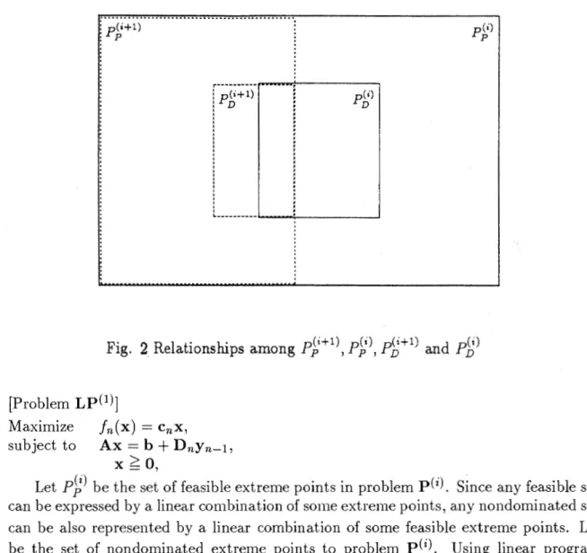
Fig.

2

Relationships among

Pp

,

P?,

P!")

and

PP

[Problem

L P ( ' ) ]

Maximize

fn(x)

= c n x , subject to

AX

=

b

+

Dnyn-1,

X

>

0,

Let

P-p'

be the set of feasible extreme points in problem

P(').

Since any feasible solution can be expressed by a linear combination of some extreme points, any nondominated solution

( 2 )

can be also represented by a linear combination of some feasible extreme points. Let

Pn

be the set of nondominated extreme points to problem

P^.

Using linear programming theory and the results of analysis given by Wen [4] and Wang et al. [3], we can represent the relationships among these sets as follows:

(1)

[Property l]

Py

C

P!)

a,nd

P(')

C

P};-",i = 2,3,.

.

.n.

[Property 21 If both a E

PP

and

a

E

P!)

hold, then a E

p f l )

holds for

i

= l ,

2 , .

. .

, n - l . Conversely,

if

a E

PP

holds, then a E

PP

holds but a E

P$'

does not always hold for

i

= 1,2,

. . .

,nà 1.

For simplicity, consider a multiobjective, two level (n =

2)

decentralized system. The original problem defined by Eqs.(l) through (13) with n = 2 is decomposed into prob- lems

P(')

and

LP(')

as defined by Eqs.(32) through (40) with n = 2. It is obvious that

P ~ I

PP

a,nd

P p 1

C

P^.

In problem the second level problem gives the set of

bases (the extreme points) with respect to X corresponding to the given vector

yl

to the first level problem. The first level constructs the set of feasible extreme points by uniting the set of fea,sible extreme points with respect to

yl

and the set of bases with respect to X

Algorithm for Multiobjective, Multilevel LP 181

provided from the second level problem. Nondominated extreme points are defined for this set of feasible extreme points and generated by searching each feasible extreme point in this

set successively. Therefore,

~ ' 2 )

PP)

holds, that is, the nondominated extreme points are

also feasible extreme points in problem

G)

(Â¥'+l ('+l) and

pn

According to properties 1 and 2, the relationships among

Pp

_,

_Pp

_,

_Pn

can be illustrated in Fig. 2.

(2)

Using the "two-level simplex algorithm [3]", we can find all the elements of the set

Pp

.

According to Property 3, we can get all the elements of the set

PP

as the elements of

P?

satisfying the optimality conditions for problems

LP('),

LPW,.

. .

,

LP("').

Note that

unlike the general multi-objective linear programming

[ 5 ] ,

it is impossible to judge whether

or not each element in

P P

is nondominated for problem

P(")

by making a local judgement

(i.e., solving a sub-LP problem) at each extreme point in

PP

on the searching process.

This is because a nondominated solution to problem is not always feasible for problem

P*")

and a dominated solution in problem can be nondominated for problem P(")

(

as indicated in Property

2.

Therefore, if an element, a, in

P})

does not belong to

pp"',

some extreme points dominated by the a in problem

P^

can be nondorninated solutions t o

problem

P(").

Fortunately, using Zeleny's theory of multi-objective linear programming [ 5 ] ,

we can construct a set of domination trees which represent domination relationships between

(2)

any pair of extreme points adjacent to each other in

Pp

.

If an a in

P )

belongs to

PP),

the a is nondominated solution to problem

P(")

according to Property 2. Otherwise, all the

extreme points dominated by the a in

PP

can be generated through the domination trees,

and should be checked whether or not they belong to

P P .

If

we can find some extreme

points belonging to

P'

on this checking process, then these points become candidates for

nondominated solutions to problem

P*").

The detailed solution procedure is presented in

section

4.

In order to generate a set of domination trees, we have to derive additional properties

with respect to extreme points in problem

P^).

For this purpose, we construct the following

problem M L P which is equivalent to P('*: [ P r o b l e m M L P ] 1 Minimize - f l ( z ) = u z , L Minimize -

f

L (z) = u z, subject to Q z = p,

'SO,

Y,

S O , x i j

S O , J ' =

1 , 2

,...,

n i , ! = 1 , 2

,...,

K ,

where

Q,

z, p and ul(row vectors),

l

= 1 , 2 , .

. .

, L ,

are defined by

G1

1

-D2

0

G 2

I

-D3

0

Gs

I

S..

-Dn-1

0

I

0

-Dn

0 A

T T T T T T T T

z =

( Y I , S 1 ,Y2,s2,...,Y,,.-l,sn,-l,x

1

7 T T p = (Y^,Y^ .+S,

~ ^ - , , b

)

,

182

Z.-

W. Wang,

H

Nagasawa &

N.

Nishiyama

where LLT" denotes the transposition and Si,

i

= l , 2,

. .

.

,

n - 1, are the slack variables for Eqs. (3), (6)) (9).

Since the feasible region of problem

MLP

is made by combining Eqs. (3)) (4)) (6))

(7))

(g),

(10))

(12)

and (13)) any feasible solution in problem M L P satisfies condition (a). How- ever, in problem M L P , the objective functions of the lower level problems are all removed and therefore a feasible solution in M L P does not always satisfy conditions (b) and (c).

A

simplex tab lea,^ for problem M L P can be constructed by using the following equations:

where

pk

and ii: are defined as

Pi

= (Qfllp)t, qi[j] =

( Q & Q N ) ~ ~ ~ ~

7

- - 1 - 2

"[j]

-

( U ~ ~ Q ~ ' Q N ) ~ ~ ~ = (uj,

-

7

where "B" and "N" stand for "basic" and "non-basic", respectively.

Letting

11

be an index set of nonbasic variables in the simplex tableau, we define

( 2 )

Consider that the current extreme point in

MLP

belongs to

Pp

.

Applying the results derived by Zenely [5] to this case, we get the following properties:

[Property 41 Assume

Oj

>

0 and u j

S

0 for a nonbasic variable, zj, j 6

11.

If the adjacent extreme point generated by introducing zj as a new basic variable belongs t o

P

,

!

then it dominates the current extreme point.

[Property 51 Assume (?j

>

0

and iij

2

O for a nonbasic variable, ~ j , j E

11.

The adjacent extreme point generated by introducing z j as a new basic variable is dominated by the current extreme point.

[Property 61 Assume that OjU,

2

Okuk for two nonbasic variables z j and zk, j,

k

6

11.

If the adjacent extreme point generated by introducing z j as a new basic variable belongs to

P',

then it dominates the adjacent extreme point generated by introducing zk as a new basic variable.

( 2 )

Using Properties 4 through 6, we can construct a set of domination trees for

Pp

.

Searching each extreme point downward from the top of each domination tree, we can find

("1

an extreme point ra,nked at the first highest level along a domination tree belonging to

Pp

.

Then all the lower-ra,nked extreme points ca,n be neglected without any search because they are explicitly dominated by the extreme point, reducing the computation time for checking whether they belong to

PP

or not. If we cannot find such an extreme point along a domination tree, all extreme points along the tree cannot become nondominated solutions to problem

pin).

Algorithm for Multiobjective, Multilevel LP 183

4. S o l u t i o n M e t h o d

We can not apply the existing methods developed for solving a usual multi-level system to generate a set of nondominated solutions to problem

P(").

We have to develop a new method exploiting Properties

1

through

6.

From Property 1, any nondominated solution to problem

P("),

equivalently any element in

PP,

not only belongs to

PE

but also belongs to

PP.

However, from Property

2,

it does not always belong to

P".

Therefore, enumeration of all elements in

Pf'

itself does not solve problem

P(").

Additional information on the rela>tionships among extreme points adjacent to each other in

PP,

such as domination trees, is helpful to generate all t h e nondominated solutions to problem

P(").

In the same way as that proposed for solving a single objective, two-level decentralized system, we can find all the extreme points in

PP'

by using the "two-level simplex algorithm

[3]."

Incorporating Properties

4

through

6

into the two-level simplex algorithm, we can provide not only all the extreme points in

PP

but also the set of domination trees. If any nond~mina~ted solution to problem listed at the top of each domination tree satisfies

(

condition (b), then it belongs to

P;).

Otherwise, the corresponding domination tree should be searched to find the first highest-ranked element along the domination tree satisfying condition (b). It should be noted that

if

the element satisfying condition (b) is not listed at the top of the corresponding domination tree, the element is not always a nondominated solution to problem P("), because it is not guaranteed for the element to satisfy condition (c). Condition (c) still remains to be checked a t the last stage of the searching procedure. This final check can be achieved by comparing the values of headquarters-objective function vector of the element with those of all the elements generated.

We summarize the proposed algorithm for generating the set of nondominated solutions to problem

P("*

as follows:

(2)

< S t e p l > Make the set of domination trees over all the extreme points of

Pp

,

by applying the two-level simplex algorithm to problem

P^

and by using properties 4 through 6.

< S t e p

2>

Along each domination tree, find the first highest-ranked element satisfying the optimality conditions for problems

L P ( ~ ) ,

,

If the domination tree ha,s some branches, find such an element along each branch. If there is no such element found, abandon the tree or branch, and proceed the search for the other trees.

< S t e p

3>

Comparing the va,lues of hea,dqua,rters-objective function vector among the ele- ments found in Step 2, generate the set of nondominated solutions to problem

P(").

5. N u m e r i c a l E x a m p l e

To show the effectiveness and applicability of the proposed algorithm, we demonstrate a numerical example. Consider a corporation consisting of one headquarters and two division each of which has two fa,ctories. Assume that the corporation produces ten kinds of products. Each factory produces two or three kinds of product denoted by xll = ( x l l l , x l 1 2 ) for the (1,l) factory, xi2 = ~ 1 2 2 , x12qT for the (1,2) factory, x21 = (a-211, x212)T for the

(2,l)

factory and x 2 2 = ~ 2 2 2 , for the (2,2) factory. We can formulate the three-level decentralized system as follows:

[ E x a m p l e P r o b l e m

<

t h e h,ea,dqua,rters p r o b l e m

>

184 Z.-W. Wang, H. Nagasawa & N. Nishiyama

y

2

0, < t h e (1, l} f a c t o r y problem> Maximize 211 =

( 2 , 3 ) x n ,

2 0

subject to

(;

;)

xi1

S

(q

3 4

200

X11

2

0, < t h e ( l , 2 ) f a c t o r y problem> Maximize

Z12

=

(1,4,2)x12,

4 subjectto

(:

10

? 0 ) ~ 1 2 5 ( ~ ! ) + ( ~ : ) Y I ,

10 20

5

X12

2

0, <th,e

2nd

d i v i s i o n problem,> ~ a x i m i z e 2 2 =

(l,2)x21 ( ~ 2 )

+

( 5 , 9 , 3 ) ~ 2 2 ( ~ 2 )

-

( l , 2 ) ~ 2 ,

9

4

28 20.5

subject to

(;

;o)

y2

5

(g)

+

(!:

i:

)

W ,

Y2

2

0 ,

<th,e

(2,1}

f a c t o r y problem,> Maximize

Z21

=

( l , 3)x21,

X21

2

0 ,

<th,e

(2,2}

f a c t o r y problem> Maximize =

( l , I , l)x22,

subjectto

(i

i ) x 2 2 ~ ( F ) + ( : i : : ) ~ 2 , X22

2

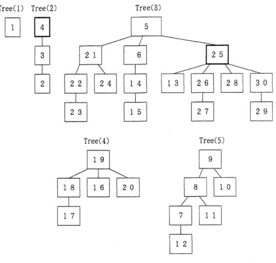
0, (2)

Using the algorithm proposed in section 4, we can

find

all the extreme points in

Pp

Algorithm for Multiobjective, Multilevel LP

0 0 0 C T 0 0 0 0 0 0 0 0 0 0 0 0 0 0 0 0 0 0 0 0 0 0 0 0 0 0

and 25 alon these element

Fig.

3

Domination t r e e s f o r t h e example problem

S satisfy the condition (b), we finally obtained elements

4

g trees

(2)

and (3). The other trees have no element satisfying condition (b). Comparing the v a l ~ ~ e s of headquarters-ob jective-functio~~ vector among these two elements, we get elements 4 and

25

as the set of nondominated solutions to problem In this case,

30

elements in

PP)

are generated, but only

22

elements are checked to judge whether or not satisfy condition (b). Domination trees are helpful to reduce a large a~nount of computatio~l effort for achieving this final check. Computation time is only about l minute by

EPSON

PC-286 without a mat hemat ical processor.

This paper discussed a mathematical model and its solution method for a multi-objective, multi-level decentralized system. An optimal solution method based on the two-level sim- p l e ~ algorithm with domination trees was proposed for solving this type of multi-level de- centralized system.

A

numerical example was demonstrated to show the effectiveness of the proposed method.

References

[l] Anandalinga,m,

G:

A

mathematical Programming Model of Decentralized Multi-Level systems.

J.

Operational Research Society, 39(1988),

1021-1033.

Algorithm for Mulr~object~ve, Multilevel LP 187

[2] Wang,

2 .

W., H. Nagasawa and N. Nishiyama, Optimal Resource Allocation in a Three-

level Decentralized System. Bulletin

of

Unzversity

of

Osaka Prefecture, Series A, 41(1992),

no. 5, 57-68.

[3] Wang,

2.

W., H. Nagasawa and

N.

Nishiyama, A New Method for Solving a Linear

Two-level Decentralized Problem. J.

of

the Operations Research Soczety

of

Japan, Vol.

38, No. 3(1995), 345-354, in Japanese.

[4]

Wen,

U. P.

and

S.

T. Hsu, Linear Bi-level Programming Problems

-

A Review.

J.

of

the Operatzonal Research Soczety, Vol. 42, No. 2(lggl), 125-133.

[5] Zeleny, M., Linear Multiob jective Programming. Chapter 3, Springer-Verlag, Berlin and

N.Y., 1974.

Hiroyuki Na,gasawa

Department of Industrial Engineering

College of Engineering

Osaka Prefecture University

1-1 Gakuen-cho, Sakai, Osaka, 580, Japan

E-mail: ngQie.osakafu-u.ac.jp