A TOPSIS-BASED ENTROPIC REGULARIZATION APPROACH FOR SOLVING FUZZY MULTI-OBJECTIVE NONLINEAR PROGRAMMING PROBLEMS

Vol. 55, No. 4, December 2012, pp. 235–244

A TOPSIS-BASED ENTROPIC REGULARIZATION APPROACH FOR SOLVING FUZZY MULTI-OBJECTIVE NONLINEAR

PROGRAMMING PROBLEMS

Fung-Bao Liu Cheng-Feng Hu

I-Shou University

(Received December 3, 2011; Revised October 10, 2012)

Abstract In this work, a version of the technique for order preference by similarity ideal solution (TOPSIS) with entropic regularization approach is developed for solving the fuzzy multi-objective nonlinear program-ming (MONLP) problems. Applying the basic principle of compromise of TOPSIS, the fuzzy MONLP problem can be reduced into a fuzzy bi-objective nonlinear programming problem. Moreover, following the “tolerance approach,” the solution of the fuzzy bi-objective nonlinear programming problem can be obtained by solving a min-max problem. An entropic regularization approach is then applied for solving such a problem. Computational results are provided to illustrate the validity and efficiency of the proposed method.

Keywords: Fuzzy sets, multiple objective decision making, TOPSIS, entropic regular-ization

1. Introduction

In the last two decades, one of the most rapidly developing methodologies is multi-criteria decision analysis of which multi-objective decision makings (MODM) plays a major role. It is well known that most decision making problems have multiple objectives which cannot be optimized simultaneously due to the inherent incommensurability and conflict between these objectives. Thus making a trade off between these objectives becomes a major subject to get the best compromise solution. A variety of methodologies for solving MODM problems have been proposed [11, 13, 15–17, 19, 20]. Among them, the goal programming and global criterion method are some of the most popular approaches. The methods only consider the criterion of the shortest distance from the given goal or the positive ideal solution. However, in practice, we might like to have a decision which not only makes as much profit as possible, but also avoids as much risk as possible. The single criterion of the shortest distance from the positive ideal solution is then not enough to satisfy decision maker(s) [9]. The technique for order preference by similarity ideal solution (TOPSIS) was first developed by Hwang and Yoon [10] to solve a multiple attribute decision making (MADM) problem. It provides the principle of compromise that the chosen alternative should have “the shortest distance from the positive ideal solution (PIS)” and “the farthest distance from the negative ideal solution (NIS).” Lately, this principle of compromise has also been suggested by Hwang et al. [9] for solving MODM problems. Recently, Abo-Sinna [1] extends the TOPSIS to solve multi-objective dynamics programming problems. Deng et al. [5] formulate the inter-company comparison process as a multicriteria analysis model, and presents an effective approach by modifying TOPSIS for solving such problem. Since vague concepts frequently represented in decision data for modeling real-life situations, multi-objective decision makings in a fuzzy

environment becomes an important problem both in theory and practice. Chen [4] extends the concept of TOPSIS to develop a methodology for solving multi-person multi-criteria decision-making problems in fuzzy environment. Inspired and motivated by the recent research, in this study, a version of the TOPSIS with entropic regularization approaches is developed for solving the fuzzy MODM model in view of the following fuzzy multi-objective nonlinear programming problem (MONLP):

Max/Min F (x) = [f1(x),· · · , fk(x),· · · , fK(x)]

s.t. (x, µ_X˜(x))∈ ˜X ≜ {(x, µ_X˜(x))| gs(x)∼ 0, s = 1, · · · , m},≤

(1.1)

where µ_X˜(·) is the membership function of the fuzzy set ˜X, gs(x) ∼ 0, s = 1, 2, · · · , m,≤

are fuzzy inequalities and “∼” denotes the fuzzified version of “≤” with the linguistic≤ interpretation “approximately less than or equal to.” Each fuzzy inequality gs(x) ∼ 0≤

actually determines a fuzzy set ˜Cs, whose membership function is denoted by µgs. The

membership grade µgs(x) can be interpreted as the degree to which the regular inequality

gs(x) ≤ 0, s = 1, 2, · · · , m, is satisfied. To specify the membership functions µgs, it is

commonly assumed that µgs(x) should be 0 if the regular inequality gs(x) ≤ 0 is strongly

violated, and 1 if it is satisfied. This leads to a membership function in the following form:

µgs(x) =    1, if gs(x) ≤ 0, µs(gs(x)), if 0 < gs(x)≤ ts, 0, if gs(x) > ts, (1.2)

for s = 1, 2,· · · , m, where ts ≥ 0 is the tolerance level which a decision maker can tolerate in

the accomplishment of the fuzzy inequality gs(x) ≤

∼ 0. We usually assume that µs(gs(x))∈

[0, 1] and it is continuous and strictly decreasing over [0, ts].

Applying the basic principle of compromise of TOPSIS, the fuzzy MONLP problem (1.1) can be reduced into a fuzzy bi-objective nonlinear programming problem. Moreover, following the “tolerance approach” [12, 21], the solution of the fuzzy bi-objective problem can be obtained by solving a min-max problem. An entropic regularization approach is then applied for solving such a problem. The rest of the paper is organized as follows. In Section 2, the TOPSIS with entropic regularization approach for solving the fuzzy MONLP will be presented. A solution algorithm and the implementation issue on the algorithm will be discussed in section 3. Some numerical results are provided in section 4. The paper is concluded in section 5.

2. TOPSIS for Solving the Fuzzy Multi-Objective Nonlinear Programming Problem

To solve the fuzzy MONLP problem (1), the principle of compromise that the chosen solution should have “the shortest distance from the positive ideal solution (PIS)” and “the farthest distance from the negative ideal solution (NIS)” is adopted. Since conflict between the distance from PIS and the distance from NIS is usually existing, a compromise cannot be simultaneously obtained with the shortest distance from PIS and the farthest distance from NIS. And, unlike MADM, MODM always has an infinite number of alternatives. It becomes impossible to find the solution with the shortest distance from PIS and the longest distance from NIS. Thus both criteria of “the shortest distance from PIS” and “the farthest distance from NIS” are substituted by “as close to PIS as possible” and “as far away from NIS as possible” [9].

To mathematically formulate this principle of compromise, we first define the reference points of PIS and NIS for the fuzzy MONLP problem as follows:

f_k∗ = max (x,µ_X˜(x))∈ ˜X fj(x) ∀ j ∈ J, = min (x,µ_X˜(x))∈ ˜X fi(x) ∀ i ∈ I, ∀ k = 1, 2, · · · , K, (2.1) f_k− = min (x,µX˜(x))∈ ˜X fj(x) ∀ j ∈ J, = max (x,µX˜(x))∈ ˜X fi(x) ∀ i ∈ I, ∀ k = 1, 2, · · · , K, (2.2)

where J denotes the index of objectives for maximization, fj(x) denotes the benefit

objec-tive for maximization,∀ j ∈ J, I denotes the index of objectives for minimization, fi(x)

de-notes the cost objective for minimization,∀ i ∈ I. Let f∗ ≜ {f₁∗, f₂∗,· · · , f_K∗} be the solution vector of equation (2.1) which consists of individual best feasible solutions for all objectives. f∗ is called the positive ideal solution (PIS). Similarly, let f− ≜ {f₁−, f₂−,· · · , f_K−} be the solution vector of equation (2.2) which consists of individual worst feasible solutions for all objectives. f− is called the negative ideal solution (NIS).

To measure the distance from PIS and the distance from NIS for each objective, the Minkowski’s Lp-metric is employed. The Lp-metric defines the distance between two points

fk(x) and fk∗ (or fk−), k = 1, 2,· · · , K. Moreover, because of the incommensurability among

objectives, the component distance from PIS or NIS for each objective is normalized. The following distance functions are then considered.

dP IS_p (x) = { ∑ j∈J wp_j [ f_j∗− fj(x) f_j∗− f_j− ]p +∑ i∈I wp_i [ fi(x)− fi∗ f_i−− f_i∗ ]p}1/p (2.3) and dN IS_p (x) = { ∑ j∈J wp_j [ fj(x)− fj− f_j∗− f_j− ]p +∑ i∈I wp_i [ f_i−− fi(x) f_i−− f_i∗ ]p}1/p , (2.4) where dP IS

p and dN ISp are the distances from the PIS and NIS, respectively, wk, k = 1, 2,· · · ,

K, are the relative importance (weights) of objectives, i.e., wk indicates the degree of

im-portance of the k-th objective, and p = 1, 2,· · · , ∞ is the parameter of distance functions. The parameter p plays the role of the “balancing factor” between the distance dp and the

objects; as p increases, the distance dp decreases, i.e., d1 ≥ d2 ≥ · · · ≥ d∞, and greater

emphasis is given to the largest deviation in forming the total. Specifically, p = 1 implies an equal importance (weights) for all these deviations, while p = 2 implies that these de-viations are weighted proportionately with the largest deviation having the largest weight. Finally, for p =∞, the largest deviation completely dominates the distance determination [10, 17, 19, 20].

To approximately minimize dP IS_p , and approximately maximize dN IS_p , the fuzzy MONLP problem can be converted to the following fuzzy bi-objective nonlinear programming prob-lem. ˜ min dP IS p (x) ˜ max dN IS p (x) s.t. gs(x)∼ 0, s = 1, · · · , m,≤ (2.5)

where p = 1, 2,· · · , ∞. The membership functions µ1(x) and µ2(x) of the two distance

objective function are assumed to be non-increasing/non-decreasing monotonous functions and can be described as follows.

µ1(x) =        1, if dP IS p (x) < (dP ISp )∗, (dP IS p )′− dP ISp (x) (dP IS p )′− (dP ISp )∗ , if (dP IS p )∗ ≤ dP ISp (x)≤ (dP ISp )′, 0, if dP IS p (x) > (dP ISp )′, (2.6) µ2(x) =        1, if dN IS_p (x) > (dN IS_p )∗, dN IS p (x)− (dN ISp )′ (dN IS p )∗− (dN ISp )′ , if (dN IS_p )′ ≤ dN IS_p (x)≤ (dN IS_p )∗, 0, if dN IS p (x) < (dN ISp )′, (2.7) where (dP IS_p )∗ = min x∼X∈

dP IS_p (x) and the solution is xP IS, (2.8) (dN IS_p )∗ = max

x∼X∈

dN IS_p (x) and the solution is xN IS, (2.9)

(dP IS_p )′ = dP IS_p (xN IS), (2.10)

(dN IS_p )′ = dN IS_p (xP IS). (2.11)

Let a fuzzy decision ˜D of the fuzzy MONLP problem be defined as the fuzzy set resulting from the intersection of fuzzy objectives and fuzzy constrains ˜Cs, s = 1, 2,· · · , m, with a

corresponding membership function µ_D˜(x) = min

s=1,2,··· ,m{µ1(x), µ2(x), µgs(x)}. (2.12)

According to reference [12, 21], a solution, say x∗, of the fuzzy MONLP problem with a degree of satisfaction, µ_D˜(x∗), can be taken as the solution with the highest membership in

the fuzzy decision set ˜D and obtained by solving the following problem:

max min

s=1,2,··· ,m{µ1(x), µ2(x), µgs(x)} (2.13)

or

− min µ′_D˜(x)≜ max

s=1,2,··· ,m{−µ1(x),−µ2(x),−µgs(x)}. (2.14)

One major difficulty encountered in developing solution methods for solving the min-max problem (2.14) is the non-differentiability of the max function µ′_˜

D(x). A distinct feature of the

recent development centers around the idea of developing “smooth algorithms” [6, 8]. Among them, a class called “regularization methods” has been developed based on approximating the max function µ′_˜

D(x) by certain smooth function [2, 3, 8]. Here we adopt the newly

proposed “entropic regularization procedure” [7, 14]. This procedure guarantees that, for an arbitrarily small ε > 0, an ε-optimal solution of the min-max problem (2.14) can be obtained by solving the following problem:

− min µq(x) = 1 q ln{exp[q(−µ1(x))] + exp[q(−µ2(x))] + m ∑ s=1 exp[q(−µgs(x))]}, (2.15)

with a sufficiently large q.

It should be noted that in practice a sufficiently accurate approximation can be obtained by using a moderately large q [14]. Also because of the special “log-exponential” form of µq(x), most over-flow problems in computation can be avoided.

3. An Algorithm and the Implementation Issue on the Algorithm

Based on the discussion in Section 2, a TOPSIS-based entropic regularization algorithm for solving the fuzzy MONLP is developed in this section.

Algorithm:

Step 0.1 Determine the distance parameter p. If the decision maker emphasizes the sum

of individual distances (regrets for dP IS_p and rewards for dN IS_p ), he should choose p = 1. On the other hand, if dominating criteria are the maximum of individual regrets and the minimum of individual rewards, p = ∞ should be chosen. Beyond both extreme cases, p = 2 will be chosen. p = 2 is similar to the popular least-square approach, and provides an approximation for the case 2 < p < · · · < ∞. Note that p = 1, 2, and ∞ are well-known standard values in the fields of control theory and multi-criteria decision making [19].

Step 0.2 Determine the relative importance wk of the K objective functions. There are

various methods for assessing wk, such as eigenvector, weighted least square, entropy and

LINMAP methods [10]. In this study, we assume that wk is given from decision makers.

Step 1. Determine the positive ideal solution (f∗) and the negative ideal solution (f−) by solving equations (2.1) and (2.2).

Step 2. Solve equation (2.5). Step 2.1 Obtain (dP IS p )∗, (dN ISp )∗, (dP ISp ) ′ and (dN IS p ) ′ by solving equations (2.8)-(2.11). Go to Step 2.2.

Step 2.2 Obtain membership functions µ1(x) and µ2(x) by calculating equations (2.6)

and (2.7). Go to Step 2.3.

Step 2.3 Solve equation (2.15). Go to Step 3.

Step 3 If the solution obtained by the TOPSIS-based entropic regularization approach is

satisfied, i.e., the degree of satisfaction obtained in Step 2.3 reaches a preference value, say ¯

α, stop. Otherwise, decision makers may like to change p, wk, q, ¯α and/or membership

functions. Then, we will go back to Step 0.1, Step 0.2, or change the tolerance levels ts, s = 1, 2,· · · , m, in (1.2). The solution procedure is then repeated.

3.1. Implementation issue on the algorithm

In step 1 and step 2.1 of the proposed algorithm, we face the challenge of solving problems (2.1), (2.2), and (2.8)-(2.11). Consider the problem in (2.1).

max fk(x) s.t. (x, µ_X˜(x))∈ ˜X, (3.1) or equivalently, max fk(x) s.t. gs(x) ≤ ∼ 0, s = 1, 2, · · · , m. (3.2)

For α∈ [0, 1], consider the following problem: max fk(x)

s.t. x∈ Xα,

(3.3) where Xα ={x | µgs(x)≥ α} is the α-level set of ˜X. Since µgs(x)∈ [0, 1] and it is continuous

and strictly decreasing over [0, ts], problem (3.3) is equivalent to the following problem:

max fk(x)

s.t. gs(x) ≤ µ−1gs (α), s = 1, 2,· · · , m, α ∈ [0, 1].

This is a parametric programming and can be solved with continuous changes of α within [0, 1]. Alternatively, we may present a list of the results to the decision maker by incremental changes of α = 0, 0.1,· · · , 0.9, 1.

A Similar argument holds for solving the problems (2.2), and (2.8)-(2.11). In this study, we assume that the value of α∈ [0, 1] is subjectively given from decision makers for obtaining the values of f_k∗, f_k−, (dP IS

p )′, (dP ISp )∗, (dN ISp )′, and (dN ISp )∗.

4. A Numerical Example

In this section, a numerical example is provided to illustrate the validity and efficiency of the proposed method.

Consider the following fuzzy multi-objective nonlinear programming problem: max f1(x) = 10x1− x21+ 6x2− x22− 2x3− 2x23+ 0.5x2x3

min f2(x) = 3x1+ 2x2− 6x1x3

s.t. g1(x) = 4x1+ 2x2+ x3− 10∼ 0,≤

g2(x) = 2x1+ 4x2+ x3− 20∼ 0, x≤ 1, x2, x3 ≥ 1,

(4.1)

with the membership functions µgs(x), s = 1, 2, are specified as follows:

µg1(x) =        1, if g1(x)≤ 0, 1− ( g1(x) 7 )2 , if 0 < g1(x)≤ 7, 0, if g1(x) > 7, µg2(x) =        1, if g2(x) ≤ 0, 1− ( g2(x) 10 )2 , if 0 < g2(x)≤ 10, 0, if g2(x) > 10.

Step 1. Let ˜X =△ {gi(x) ∼ 0, i = 1, 2, and x≤ 1, x2, x3 ≥ 1}. Determine the positive ideal

solution (f∗) and the negative ideal solution (f−) by solving the following problems: f₁∗ = max x∈ ˜X f1(x) = 10x1− x21+ 6x2− x22− 2x3− 2x23+ 0.5x2x3, _(4.2) f₂∗ = min x∈ ˜X f2(x) = 3x1+ 2x2 − 6x1x3, _(4.3) f₁− = min x∈ ˜X f1(x) = 10x1− x21+ 6x2− x22− 2x3− 2x23+ 0.5x2x3, _(4.4) f₂− = max x∈ ˜X f2(x) = 3x1 + 2x2− 6x1x3. _(4.5)

To solve the problem (4.2), for α∈ [0, 1], we consider the following parametric programming problem:

max f1(x) = 10x1− x21+ 6x2− x22− 2x3− 2x23+ 0.5x2x3

s.t. 7√1− α − 4x1− 2x2− x3+ 10≥ 0,

10√1− α − 2x1− 4x2− x3+ 20 ≥ 0, x1, x2, x3 ≥ 1.

(4.6) By incremental changes of α = 0, 0.1,· · · , 0.9, 1, the solution of the problem (4.6) at α can be obtained as shown in Table 1. Taking α = 0.9, the results for solving problems (4.3), (4.4), and (4.5) are shown in Table 2. Next, we compute dP IS

p and dN ISp and obtain the

following equations: dP IS_p = ( wp₁ ( 19.8788− f1(x) 19.8788− (−72.5379) )p + wp₂ ( f2(x)− (−33.3827) 4.2136− (−33.3827) )p)1/p , dN IS p = ( w₁p ( f1(x)− (−72.5379) 19.8788− (−72.5379) )p + w₂p ( 4.2136− f2(x) 4.2136− (−33.3827) )p)1/p .

Table 1: The solution, x∗, of the problem (4.6) at different α∗ α x f₁∗ 0 (2.9000, 2.2000, 1.0000) 26.0500 0.1 (2.8282, 2.1641, 1.0000) 25.6640 0.2 (2.7522, 2.1261, 1.0000) 25.2467 0.3 (2.6713, 2.0857, 1.0000) 24.7841 0.4 (2.5844, 2.0422, 1.0000) 24.2688 0.5 (2.4899, 1.9950, 1.0000) 23.6871 0.6 (2.3854, 1.9427, 1.0000) 23.0176 0.7 (2.2688, 1.8834, 1.0000) 22.2246 0.8 (2.1261, 1.8130, 1.0000) 21.2384 0.9 (1.9427, 1.7214, 1.0000) 19.8788 1 (1.5000, 1.5000, 1.0000) 16.2500

Table 2: The results for solving problems (4.3), (4.4), and (4.5)

Problem x objective value

Problem (4.3) (1.2142, 1.0000, 5.3568) f₂∗ =−33.3827 Problem (4.4) (1.0000, 1.0000, 6.2136) f₁− =−72.5379 Problem (4.5) (1.0000, 3.6068, 1.0000) f₂− = 4.2136

Step 2. For w1 = w2 = 1₂ and p = 2, solve the following problem:

˜ min dP IS 2 (x) ˜ max dN IS₂ (x) s.t. x ∈ ˜X. (4.7) Step 2.1. Obtain (dP IS 2 )∗, (dN IS2 )∗, (dP IS2 ) ′ and (dN IS 2 ) ′

by solving the following problems: (dP IS

2 )∗ = min x∈ ˜X

dP IS

2 (x), (4.8)

and the solution is xP IS _{= (1.7987, 1, 3.0187).}

(dN IS

2 )∗ = max x∈ ˜X

dN IS

2 (x), (4.9)

and the solution is xN IS _{= (1.6570, 1, 3.5857). Then, we have}

(dP IS₂ )∗ = dP IS₂ (xP IS) = 0.1650, (4.10) (dN IS₂ )∗ = dN IS₂ (xN IS) = 0.5456, (4.11) (dP IS₂ )′ = dP IS₂ (xN IS) = 0.1848, (4.12) (dN IS₂ )′ = dN IS₂ (xP IS) = 0.5426. (4.13)

Step 2.2. The membership functions µ1(x) and µ2(x) of the two distance objective function

can be described as follows.

µ1(x) =        1, if dP IS₂ (x) < 0.1650, 0.1848− dP IS 2 (x) 0.1848− 0.1650 , if 0.1650≤ d P IS 2 (x) ≤ 0.1848, 0, if dP IS 2 (x) > 0.1848, (4.14)

Table 3: The results for solving problem (4.1) with equal weights w1 = w2 = 1₂ Case f1 f2 x1 x2 x3 p = 1, min dP IS 1 max dN IS 1 −5.7952 −5.7952 −26.3948−26.3948 1.7538 1.7538 1.0000 1.0000 3.1984 3.1984 p = 2, min dP IS 2 max dN IS₂ max µ_D˜(x) −3.0015 −12.2687 −6.7392 −25.1823 −28.6780 −26.8424 1.7987 1.6570 1.6889 1.0000 1.0000 1.8701 3.0187 3.5857 3.5180 µ_D˜(x) = 0.6712 p = 10, min dP IS 10 max dN IS 10 max µ_D˜(x) −1.9400 19.8785 13.6874 −24.6806 −2.3855 −15.9142 1.8164 1.9427 2.0990 1.0000 1.7213 1.9077 2.9481 1.0000 2.0666 µ_D˜(x) = 0.6252 µ2(x) =        1, if dN IS₂ (x) > 0.5456, dN IS₂ (x)− 0.5426 0.5456− 0.5426 , if 0.5426≤ d N IS 2 (x)≤ 0.5456, 0, if dN IS 2 (x) < 0.5426. (4.15)

Step 2.3. The maximizing solution, x∗, of the fuzzy MONLP problem can be obtained by solving the following problem:

max min

x1,x2,x3≥1{µ

1, µ2, µg1, µg2}. (4.16)

This problem is equivalent to the following min-max problem: − min max

x1,x2,x3≥1{−µ

1,−µ2,−µg1,−µg2}. (4.17)

A near-optimal solution of the “min-max” problem can be obtained by solving the following problem:

− min

x1,x2,x3≥1

1

q ln{exp[q(−µ1(x))] + exp[q(−µ2(x))] + exp[q(−µg1(x))] + exp[q(−µg2(x))]},

with a sufficiently large q. In our implementation, we use a fixed q = 100, the compromise solution of the fuzzy MONLP problem (4.1) is (1.6889, 1.8701, 3.5180) with the degree of satisfaction being equal to 0.6712. Tables 3 and 4 provide results for solving the fuzzy MONLP problem (4.1) with different cases of p and weights between objectives. From the results of Tables 3 and 4, we can see that solutions of “min dP IS₁ ” and “max dN IS₁ ” are the same in both cases of equal weight (w1 = w2 = 1₂) and unequal weight (w1 = 3₄, w2 = 1₄).

It is because that dP IS

1 = 1− dN IS1 . In this case, we don’t need to solve Equations (2.13)

and (2.15). When p ≥ 2 (p = 2, 10), solutions of “min dP IS_p ” and “max dN IS_p ” are always different. For those cases of different solutions, we need to solve Equation (2.15) to obtain a compromise solution which has the shortest distance from the positive ideal solution and the farthest distance from the negative ideal solution.

5. Conclusions

In this paper, the solution of a fuzzy multi-objective nonlinear programming problem is studied. A TOPSIS-based entropic regularization approach is developed for solving the

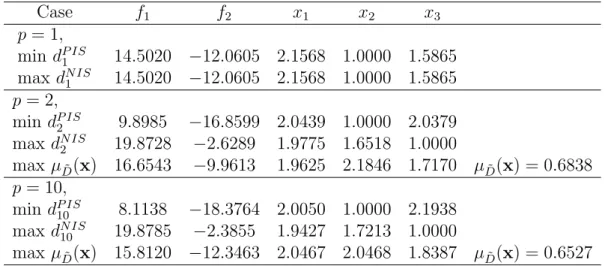
Table 4: The results for solving problem (4.1) with unequal weights w1 = 3₄, w2 = 1₄ Case f1 f2 x1 x2 x3 p = 1, min dP IS 1 max dN IS 1 14.5020 14.5020 −12.0605 −12.0605 2.1568 2.1568 1.0000 1.0000 1.5865 1.5865 p = 2, min dP IS 2 max dN IS₂ max µ_D˜(x) 9.8985 19.8728 16.6543 −16.8599 −2.6289 −9.9613 2.0439 1.9775 1.9625 1.0000 1.6518 2.1846 2.0379 1.0000 1.7170 µ_D˜(x) = 0.6838 p = 10, min dP IS 10 max dN IS 10 max µ_D˜(x) 8.1138 19.8785 15.8120 −18.3764 −2.3855 −12.3463 2.0050 1.9427 2.0467 1.0000 1.7213 2.0468 2.1938 1.0000 1.8387 µ_D˜(x) = 0.6527

fuzzy MONLP. Computational results are provided to illustrate the validity and efficiency of the proposed method. Also, because µq(x) appears in a special “log-exponential” form,

it is highly smooth and avoids most over-flow problems in computation. Compared to other approaches to solving fuzzy multiobjective programming problems, our work essentially reduces the problem to minimizing an infinitely smooth function without any constraints for efficient computation.

It should be noted that in the crisp MODM theory, only the feasible solutions are considered as candidates for efficient solutions (Pareto optimal solutions). For the fuzzy multi-objective nonlinear programming problem (1.1), however, solutions do not only differ with respect to the associated vales of the objectives, but also with respect to their degree of feasibility. In this case, the satisfactory (compromise) solution obtained by the proposed algorithm need not be nondominated.

Moreover, the max-min operator employed here is not compensatory. In this case, the satisfactory level of “as close to PIS as possible” cannot be increased by decreasing the satisfactory level of “as far away from NIS as possible.” This may be inconsistent with the basic principle of compromise of TOPSIS. Future studies should apply compensatory operators (such as min-bounded sum operator, fuzzy “and”, weighted mean operator, etc.) to obtain the compromise solution of the fuzzy MONLP problem.

Acknowledgments

The authors would like to thank referees for their constructive and valuable suggestions.

References

[1] M.A. Abo-Sinna: Extensions of the TOPSIS for multi-objective dynamic programming problems under fuzziness. Advances in Modelling and Analysis, 43-4 (2000), 1–24. [2] D.P. Bertsekas: Constrained Optimization and Lagrange Multiplier Methods (Academic

Press, New York, 1982).

[3] C. Charalammbous and A.R. Conn: An efficient method to solve the minimax problem directly. SIAM Journal on Numerical Analysis, 15 (1978), 162–187.

[4] C.T. Chen: Extensions of the TOPSIS for group decision-making under environment. Fuzzy Sets and Systems, 114 (2000), 1–9.

[5] H. Deng, C.H. Yeh, and R.J. Willis: Inter-company comparison using modified TOPSIS with objective weights. Computers and Operations Research, 17 (2000), 963–973. [6] G. Di Pillo, L. Grippo, and S. Lucidi: A smooth method for the finite minimax problem.

Mathematical Programming, 60 (1993), 187–214.

[7] S.-C. Fang and S.-Y. Wu: Solving min-max problems and linear semi-infinite programs. Computers and Mathematics with Applications, 32 (1996), 87–93.

[8] C. Gigola and S. Gomez: A regularization method for solving the finite convex min-max problem. SIAM Journal on Numerical Analysis, 27 (1990), 1621–1634.

[9] C.L. Hwang, Y.J. Lai, and T.Y. Liu: A new approach for multiple objective decision making. Computers and Operations Research, 20-8 (1993), 889–899.

[10] C.L. Hwang and K. Yoon: Multiple Attribute Decision Making: Methods and Applica-tions (Springer, Heidelberg, 1981).

[11] D. Jones, M. Tamiz, and J. Ries: New Developments in Multiple Objective and Goal Programming (Springer-Verlag, Heidelberg, 2010).

[12] Y.-J. Lai and C.-L. Hwang: Fuzzy Mathematical Programming: Methods and Applica-tions (Springer-Verlag, 1992).

[13] Y.-J. Lai and C.-L. Hwang: Fuzzy Multiple Objective Decision Making: Methods and Applications (Springer, Berlin, 1994).

[14] X.-S. Li and S.-C. Fang: On the entropic regularization method for min-max problems with applications. Mathematical Methods of Operations Research, 46 (1997), 119–130. [15] M. Ramezani, M. Bashiri, and A. C. Atkinson: A goal programming-TOPSIS approach to multiple response optimization using the concepts of non-dominated solutions and prediction intervals. Expert Systems with Applications, 38-8 (2011), 9557–9563.

[16] M. Sakawa: Fuzzy Sets and Interactive Multiobjective Optimizations (Plenum Press, 1993).

[17] R.E. Steuer: Multiple Criteria Optimization: Theory, Computation, and Application (Wiley, New York, 1986).

[18] B. Werners: An interactive fuzzy programming system. Fuzzy Sets and Systems, 23 (1987), 131–147.

[19] P.L. Yu: Multiple-Criteria Decision Making: Concepts, Techniques, and Extensions (Plenum Press, New York, 1985).

[20] M. Zeleny: Multiple Criteria Decision Making (McGraw-Hill, New York, 1982).

[21] H.-J. Zimmermann: Fuzzy Set Theory and Its Applications, 2nd Edition (Kluwer Aca-demic, Dordrecht, 1991).

Cheng-Feng Hu

Department of Industrial Management I-Shou University

Ta-Hsu, Kaohsiung 804, Taiwan E-mail: [email protected]