Light-front Tamm-Dancoff approximation and the vacuum structure of the massive Sch

九州大学学術情報リポジトリ

Kyushu University Institutional Repository

質量のあるシュウィンガー模型に対する光円錐Tamm- Dancoff近似と真空の構造

谷口, 正明

九州大学理学研究科物理学専攻

https://doi.org/10.11501/3110837

出版情報：Kyushu University, 1995, 博士（理学）, 課程博士

Light-front Tamm-Dancoff approximation and the vacuum structure of the massive Sch

^w

in g

^er

model

Masa-aki Taniguchi

Department of Physics, l(yushu Univ rsity January 5, 1996

Abstract

We investigate the massive Schwinger model quantized on the light cone with great care on the bosonic zero modes by putting the system in a finite

(

^light-cone

)

spatial box. After Dirac quantization for the constrained system, the zero mod of A+ survives as a dynamical degree of freedom. \Ve show that the physical state condition relates the fermion Fock states to the zero mode of the gauge field. We construct the physical vacuum by imposing the physical state condition carefully.

The periodicity of physics in () can be understood as that of the Bloch spectrum for the periodic "effective" potential. We calculate the B-dependence of the vacu urn energy density quantitatively and find the signal of the phase transition at () ^{= rr.}

1 Introduction

Recently there has b en growing interest in the light-front Tamm-Dancoff (L TD) approximation

[1]

as a new promising numerical approach to nonp rturbativ problern

[1-10).

It has been successfully applied to two-dimensional mod ls

[4-10),

although the application to

QC D1+3

is still beyond our control despit of much recent ffort

[2).

_{It is}

important to note that this new approach not only reproduces known results ^COlT tly, but also brings us new results

[6-9]

which have never be n obtain d by other method . (S e also Refs.

[11]

for some of such "new" results in the discr tiz d light-cone quantization (DLCQ) approach

[12].)

The LFTD approximation is the Tamm-Dancoff approximation (a truncation of the infinite dimensional Fock space by limiting the number of constituents

[13])

appli d to field theory quantized on the light cone. Th light-con quantizatio i ssential for th validity of the Tamm-Dancoff approximation: Tamm-Dancoff approximation is a kind of the valence quark approximation and on the light cone, pair creations/ annihilations are kinematically suppressed

[3],

then it is plausible that the sea quark/gluon contributions are small in this framework. Typically, the lightest particles are expected to be in the valence states. It is generally true in the rnodels so far investigated.

It has several attractive points corn pared to the lattice formulation: (j) It is based on the diagonalization of the (light-cone) Han1iltonian. It is ther for intuitively app aling, and giv s eigenvalues and eigenvectors simultaneously. (ii) One does not nc d to make

"Wick rotations" at all. Thus one may include topological terms (such as a 0-t rm) which usually cause trouble in the lattice formulation.

Th re are however some problems in light-front field theory

[3]:

(i) The vacuum prob­

lem. (It is also known as the "zero-mode problem.') In the light-cone quantization, it is not clear how the complex structure of the vacuum emerges, which is suppos d to be responsible for spontaneous symmetry breaking, the vacuum angle, etc. It is wid ly

beli ved that the zero modes of the fi ld variabl s play an important rol . (ii) The r nor-

malization problem. Even the power-counting rules are dift rent from th usual covariant ones and there are infinitely many relevant and marginal op rators

[14].

Although th r is an attempt to overcome this difficulty, we still do not know how to r norrnaliz uch theories.

A nice way to attack these difficult probl ms is to separate them each other. In thi paper we study the massive Schwinger model

( Q

E D1

+I)

in th L TD approximation, and investigate the vacuum angle, B. Since it is a two-dimensional model, we can avoid the renormalization problem and concentrate on the zero-mode problem.

The massive Schwinger model has been studied by many authors becaus it shares several important features with

QC D1+3

such as quark confinement, anomalous

U(1)A

breaking as well as B-vacuum

[4,

6,

20, 21].

In his seminal paper

[21],

Col man show d that the vacuum angle B can be regarded as an external constant electric fi ld. On of his important results is that the periodicity of physics in e is a cons quence of dynamical structure of the vacuum. Namely, it comes out from the fact that a pair cr ation of a fermion and an anti-fermion from the vacuum is energetically favorabl in a background electric field stronger than a certain critical value. He also obtains that at 0 = 1r the theory undergoes a phase transition as it passes from strong to weak coupling.

How can this dynamical feature of B be und rstood in the light-cone quantization with a sin1ple vacuu1n? The main purpose of this thesis is to xplain how the dyna1nical zero

modes of the gauge fields are related to the vacuum structure (the vacuum angle). In order to xplicitly extract the zero modes, we first put the syst m into a finit light-cone spatial box

(x-

E

[-L, L])

and impose the periodic boundary condition

[15],

keeping in mind that we should eventually take the limit

L

-+ CX). Even after fixing a gauge, th

0

zero mode of the longitudinal component of the gauge field

(A+)

r mains to be dynamical

- 0 -

while the other gauge components

(A+ ,A-,A-)

do not. We did not include the fermionic zero modes tentatively although they might be important in other respects.

The vacuum angle,() has not been discussed much in the light-cone context. Although there are several papers on the B-terrn (vacuum) in the Schwinger rnodel, the massive Schwinger rnodel has been rarely studied. Our approach may appear similar to that of Heinzl, Krusche and Werner [17], who discussed the zero modes of the gauge field in the massless Schwinger model and how the B-vacuum arises. There are, however, critical dif­

ferences; (i) Their treatment of the regularized current is not adequate. In their paper the chiral anomaly is not derived through the point-splitting regularization but as a conse­

quence of the classical equation of motion. (ii) They impose a regularized charge densjty as an additional constraint, which leads to a second-class Gauss law (the chargeless con­

dition). Of course these are different fonn the usual treatrnent of the regularized currents and the Gauss law, and they lost the dynamical zero mode A+ because of this constraint.

In this thesis, we take a great care of the relationship between the regularization of the currents and the Gauss law. We find that the regularization does not affect the structure of constraints. We end up with the first-class Gauss law and the usual chiral anomaly which arises from a gauge-invariant regularization procedure.

There are several papers on the massive Schwinger model on the light cone. Bergknoff [4] first applied the LFTD approximation and Mo and Perry [5] refined his calculations by using the method of basis functions. We have achieved six-body LFTD calculations in order to investigate two-meson and three-meson bound states [7, 8]. Eller, Pauli and Brodsky [16] considered the discretized light-cone quantization

(DLCQ)

of the massive Schwinger model. This thesis is based on these. These papers include the essence of the LFTD approximation although they did not treat the zero rnode at all. We refer the readers to them.

In Sec. 2, we review the essence of the light-front field theory and the LFTD approx­

imation, and show that the quantization on the light cone is essential for the validity of the Tamm-Dancoff approximation. We summarize our results of the 6-body

LFTD

approximation applied to the massive Schwinger model.

5

In Sec.

3,

we first examine the constraints and liminat depend nt d gr of fr dom,

paying attention to bosonic z ro modes. We find that the z ro mode of A_ and its canonically conjugate momentum remain to be dynamical. To quantiz th theory, we need to regularize operators to make them well-defined. W show that the regularization does not affect the structure of the constraints.

In Sec. 4, we investigate the ground state, namely the vacuum structure of th massive Schwinger model. The ground states are found to be infinitely degenerate. We d fine the vacuum state by making coherent superpositions of these infinite number of state . We find out the physical vacuum

(

_0-vacuum

)

by imposing the physical state condition.

Interestingly, the physical state condition relates the fermion Fock states to the zero mode of the gauge field.

Sec. 5 is devoted to the conclusion and discussions. In Appendix A, we collect th notations in this thesis and the explicit equations of the 6-body LFTD approxirnation for the massive Schwinger model. Appendix B contains a proof of the "iterativ property"

of Dirac brackets

[30),

which may be of some use when treating a syst m with many constraints. We give a detailed discussion on current regularization and chiral anomaly in Appendix C.

2 Light-front Tamm-Dancoff approximation

In this section we discuss the elementary idea of th light front field theory and the merit of the Tamm-Dancoff approximation on the light con . For simplicity w work on the two dimensional case. To higher dimensional cases also this id a is basically applicable with some trivial extensions.

The light-cone space-time is defined as a linear combination of the usual spa e-tim

(2.1)

where x0 and x1 are the (usual) time and space, respectiv ly. W call

x+

th light-cone time and x- the light-cone space. The element of the metric is

(2.2)

Usually in the equal-time quantization the momentum operator, P1, is the generator

of the translation in the spatial direction and the dynamics is described by th time­

development which is generated by the Hamiltonian, P0. In th light-con flam , the translation in the light-cone space is generated by the light-cone momentum,

p+,

and the dynamics is defin d as the light-con time development which is g nerat d by the light-cone Hamiltonian, p-.

The most important feature on the light-front field th ory is that the mom nta of particles are positive. It is easy to derive this feature for the on-shell particles:

p

2 ⁼

2p+p-

⁼ m2. The energy

p-

is always positive, and so is the momentum

p+.

For the off-shell particles it becomes almost the same situation as the on-shell case when one first integrat s the p- in the propagator

(31].

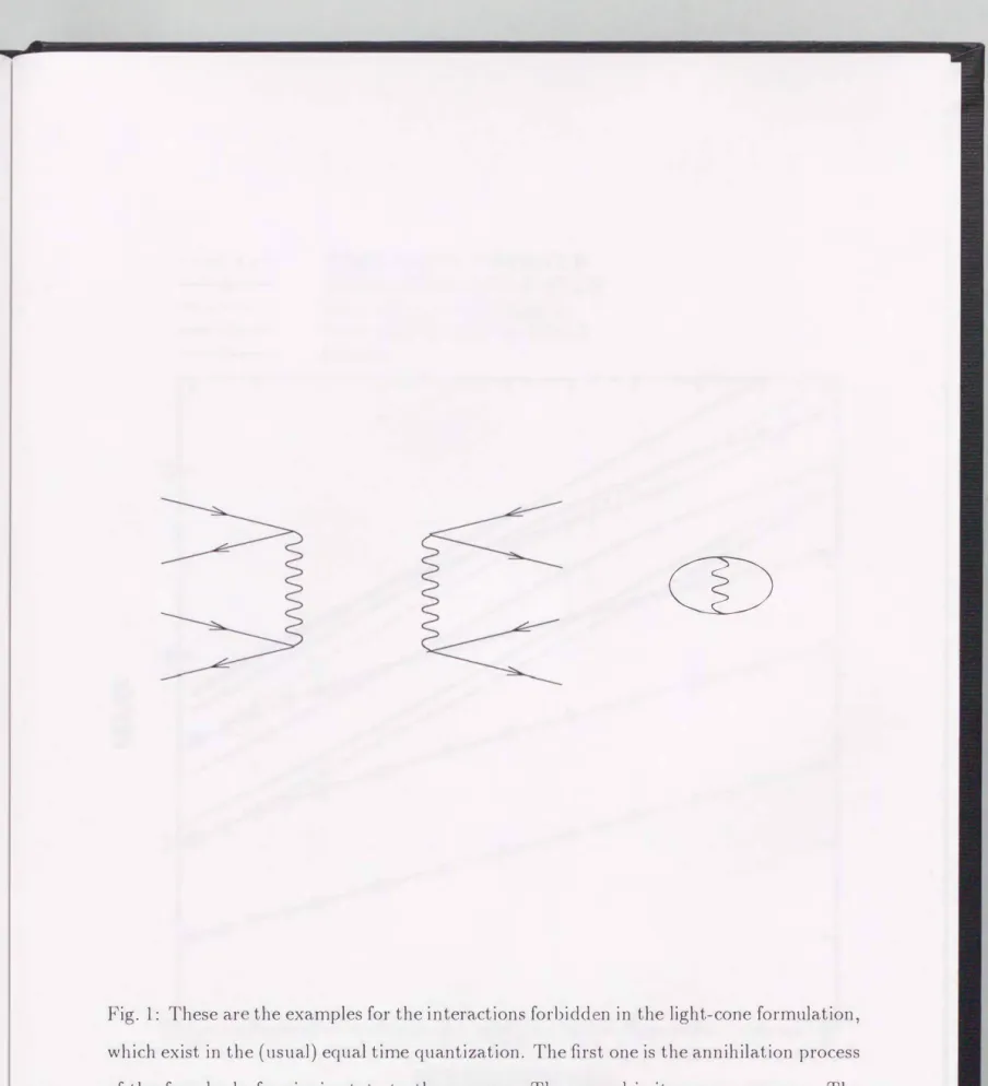
Because every momentum of the particles is positive, the pair creation( annihilation) is forbidden due to th momentun1 cons rvation.

In the same manner there exist no such interactions as four f rmions emerging( vanishing) from( into) the vacuum in the four point interactions such as the current-current Coulomb int raction or the four-Fermi interaction. In the light-con quantization scheme therefore

the vacuum decouples from the particle stat and it is usually the simpl Fock vacuum.

For example, see Fig.

^1.

In the following we solve the Einstein-Schrodinger equation:

(2.3)

where M2 is the mass-squared and 17/J(P)) is the particle state with the total momentum P. We consider the "mesonic" states in the following for simplicity. This stat 17/J( P)) is decomposed into the states with j fermions and j antifermions, l2j(P)),

17/J(P))

⁼

I2(P)) + I4(P)) + I6(P)) +... (2.4)

where the fermion number must be sa1ne as the antifermion number for th "m sonic"

state. Th se states are constructed by operating the fermion and anti£ rmion creation operator on the Fock vacuum. (See Appendix A for th explicit expressions for thes states of the massive Schwinger model.) If we investigate a model which contains th dynamical gauge fields in such a case as 4 dimensional QC

D,

w must includ the numb r of the gauge field in this decomposition.

This Einstein-Schrodinger equation is rewritten in the matrix form:

H22 H24 H26 7/;2 7/;2

H42 H44 H46 7/;4

=

M2 7/;4

(2.5)

H62 H64 H66 7/;6 7/;6

where

^Hii

consists of the kinetic energy and interactions which do not change the particle number, and Hij is an interaction which changes i particles into j particles. 7/;2, 7/;4, 7/;6,

^·

.

^.

are th wave functions of the 2-body, 4-body, 6-body,

^{· · ·}

fermionic states, resp ctively.

On the light cone, there exist no such interactions as to change th particle number by four (or more) in the four point interactions. Therefore we have th matrix element Hij

⁼ 0

for j 2: i + 4 and j::; i -4 while we would have Hij -1-

0

for j

⁼

i+4 and j

⁼

i -4 in the equal­

time quantization. The matrix of the Hamiltonian on the light cone is slimmer than that

of th equal-time quantization. To solve this equation we truncat particl numb rs, which is called the Tamm-Dancoff approximation. (In App ndix A w truncate up to including 6-body states.) After diagonalizing the Hamiltonian w simultaneously g t masses and wave functions as eigenvalues and eigenfunctions, respectively. W emphasiz that thi approximation is not based on the perturbation. Namely thi approach is nonp rturbative one. By direct diagonalization of the matrix for any value of the coupling constants, w can get the non-perturbative results.

After solving Eqn. (2.5) we must make sure that this approximation is plausible or not for the states which we look at. In the perturbative sense it is plausible that on

"mesonic" state does not have

4

fermionic component or higher because the off-diagonal elements of the matrix is proportional to the coupling constant. If the coupling constant is weak enough that the perturbation makes sense, the "mesonic" state is not affect d by the higher Fock states. For this state it is justified to truncate the Fock space only up to including 2-body state. For the strong coupling constant, it is nontrivial whether this approximation is good or not. We can make sure it by looking at obtained wave functions,

7/J2, 7/J4, 7/J6,

· · · . If

7/J4

or higher are negligibly small compared with

7/J2

for the "mesonic"

state, then the approximation is plausible for this state.

In the previous works on the massive Schwinger model

[7],

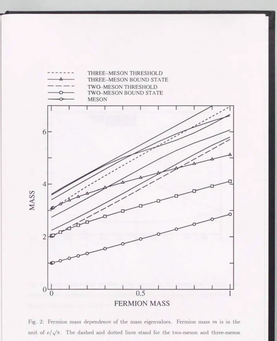
we obtained the following results by using the LFTD approximation up to including six-body states.

(1)

Th masses of the lowest states do not change if we include four- and six-body states.

(2) In particular, the state which can be regarded as a bound state of two mesons has a negligible six-body component.

(3)

W find a candidate for the bound state of three mesons.

(

4)

The wave function of the relative motion of the two-meson bound state d scribes th bound state well. We can have a picture that in the strong coupling region it is loos ly bounded, while in the weak coupling region it is tightly bounded, compared with the size of the meson.

In Fig. 2 we show the mass spectrum in th strong coupling r gion wh r th fermion rna s is given in the unit of the coupling constant

e/ fo.

We emphasize that the information about stat s

(

wav functions

)

is very u ful. It was used for identifying the three-meson bound stat . Th three-m son bound stat , if it exists, must be in the continuum spectrum unless it is light r than two m on

.

_It

IS therefore apparently difficult to identify the state among the continuum. W could however find a candidate among several states by looking at the wave functions. The point is that below the three-meson threshold, six-body compon nts should b very small except for three-meson bound states. As another example, we introduce the wav function of the relative motion in the two-meson bound state and try to describe the bound state in terms of the wave function. Although the concept of "relativ motion" of a r lativistic bound stat is somewhat awkward, we however find that the two-meson bound stat is well described in terms of the wave function of the relative motion, in the sense that a smaller set of basis functions motivated by the concept of the relative motion gives a good approximation. It gives us a qualitative picture of the bound state. The readers who ar interested in these matters, see Ref.

[7].

3 Light-cone quantization in a box

3.1 Constraints of QED2 on the light cone

In this section we analyze the structure of constraints of the massive Schwing r mod 1, including zero modes, and derive the Hamiltonian in a canonical way. In order to explicitly separate the zero modes from the non-zero modes of the bosonic variables, we put the system into a finite light-cone spatial box

(x- E ^{[-L, L])}

with the periodic boundary

condition. For the fermionic variables we impose the anti-p riodic boundary condition and disregard their zero-modes completely. W will discuss possible consequ nces of th inclu ion of the fermionic zero modes in Section

5.

The Lagrangian density of the massive Schwinger model is given by

1 -

£ ^{= -}

4

^{Fp.vpp.v +}

?f;(tP-(i8P-- eAP-)- m)?/; (3.1)

1 ^o 2

eB

^o 1 - - 2 rn t ^. t .

=

2(8+ A_)

+

27r a+ A_ +2(8+A-- a_A+)

+

v 2(?j;R't8+?fJR

+

?j;L't8_?fJL) -m(?/Jk?/JL

+

'1/Jl'I/JR)- e(h'I/Jk'I/JRA+

+

h'I/Jl'I/JLA-), (3.2)

0 -

where

A±

stands for the zero mode of

A±

and

A±

the non-z ro mode. We will use similar notations hereafter. we refer the readers to Appendix A for other notations. The conjugate momenta are obtained as follows:

(3.3) (3.4) (3.5)

Note that because the zero modes do not dep nd on x-, it is useful to extract the fac-

tor

L

from the conjugate momenta, and that, for the fermionic variables, the dagger ed/undaggered momenta are conjugate to undaggered/daggered variables, respectiv ly, e.g.,

1rk

^:=

6Lj6(8+'1fJR)·

From these we see that the primary constraints are as follows:

0

e ₁₌

-E+

_{, e 2= -}

E-+

_{, e} 3 =7rR-'lVL_{- t · r.;2�}'f'R' _,,t The total Hamiltonian[30) becomes

(3.6)

6

+

m(7/Jk7/JL

₊

7fJ17fJR)

₊

e(V27/Jk7fJRA+

₊

V27fJ17fJLA_)

₊

L ei.Xi],

(3.7)

i=l

where .-\ i ( i = 1, ... , 6) are Lagrange multipli rs. The consist ncy conditions for 83 and 84 only determine the Lagrange multipliers .-\4 and .-\3 respectively. The rest leads to further (secondary) constraints.

(3.8) (3.9) (3.10) (3.11)

The consistency conditions for these constraints do not lead to any further constraints.

(The consistency conditions of cps and c.p6 determine the multipliers .-\6 and As respectively, while those of c.p1 and c.p2 are satisfied automatically.) As usual we can arrang th s constraints into first- or second-class ones. We find the following first-class constraints,

We choose the following gauge-fixing conditions,

(3.12) (3.13) (3.14)

(3.15)

Note that the consistency of

x2

g1ves the third constraint /3· The con ist ncy of /1

and

x3

determine the multiplier )11 and

A2

r sp ctively. Inter stingly one cannot choose

0

A_� 0 because it does not have non-vanishing Poi son brack ts with any of th first-clas

constraints. We end up with a single first-class constraint <.p1, th charge. W will impose it as a physical state condition after quantization.

(

^3.16

)

which eliminates charged states from the physical space.

We use second-class constraints to eliminate dependent d grees of freedom. It is easy

0 0

to see that the independent variables are A_,

E-, 7/JR

^and

7/Jk.

Non-vanishing Dirac brackets

[

³⁰

]

for these variables are calculated as

(

^3.17

)

(

In ord r to get the Dirac brackets, one usually needs to obtain th inv rse matrix of a big matrix. his routine burden reduces considerably if we use the "iterative property". For the r aders' convenience the proof is included in Appendix

B.)

In terms of independ nt degrees of freedom, the Hamiltonian can be written as

0

pz�ro

⁼

L(E-)2,

m2 J

^{L . o}

^_

^{1 . o}

^_

p- fmass y'2

^{= _ -L}

dx-[ "

^If/

' 't (x-)e-teA_x -eteA_x R

^· _{io_} ^{,If' R 1,}

(x-)]

^'

Pi;.ter

⁼

; j_: ^dx-]+(x-) C�_) ^{2 ]+(x-),}

(

^3.18

) (

^3.19

) (

^3.20

)

(

^3.21

)

where the inverse of the derivative operator is understood as the principal value in the

0 0

Fourier transforms

[

²⁵

]

. Note that the dynamical zero modes

(A_, E-)

come into the expression in a nontrivial way. The first term

Pz�ro

is the energy of the constant el ctric

field. The second term

Pimass

contains th interaction of the z ro mode of the gauge field with the fermion, and requires a special care. It is inter sting to note that only the non-zero mode of the current appears in the third term

Pi�ter·

3.2 Current and charge regularization, and subsidiary condition

In order to quantize the theory, we replace Dirac brackets with th corresponding ( (

-i)

times) equal-x+ commutators. In addition, we need to regularize compo ite op rators to

make them well-defined. In two dimensions, on can eliminate all divergences by normal­

ord ring. In the following, we carefully defin the current operators, Hamiltonian and charge in a well-defined way so that the structure of constraints analyzed in the previous subsection is not altered by the regularization.

First of all, we have to define the "normal-ordering." For this purpose, we tr at the

0 0

gauge field

A_

(or, q =

(L/'rr)eA_,

which is nothing but the Chern-Simons term in one dimension) as an external field and quantize the fcrmionic variabl s in this external fi ld.

We make the Fourier expansion of the fermionic variable

'1/JR,

(3.22)

From the corresponding Dirac brackets,

an+l

is assum d to satisfy the following anti-

2

commutation relations,

{an+�,a � ^+t}

⁼

8n,m, {an+�, am+�}= {a � ^+t'a � ^+t}

^{= 0. Using}

these operators, we define a set of reference states, so-called "N-vacua," in analogy of Dirac sea,

(3.23)

where

IO)

is the 'empty' state, i.e.,

an+liO)

⁼ 0 for any n. At this moment, N is an

2

arbitrary int ger. (The use of the "N-vacua" is rather standard in the Schwinger model in the equal-time quantization. See Refs. [22, 23).) This state is satisfied with the nor- malization condition:

N(OIO)N'

⁼

8N,N'·

It is easy to derive the vacuum expectation value of the fermionic part of the Hamiltonian,

N(OIP�rmioniO)N'

⁼ 0 if N

=/:-

N', where

PTermion

⁼

PTmass

⁺

pc�rrent.

(The use of the

We regularize the current by point-splitting. We define the current operator

jJJ.(

x) in

a gauge invariant way

0 �

where only A_ and A+ are non-zero. A straightforward calculation shows

where

In Appendix

^C,

we discuss how to obtain the Schwinger term and th anomal vation law of the axial vector current.

(3.24)

(3.25)

(3.26)

o s r-

A problem arises when we treat zero-modes with care. Because of the relation j�

⁼

-f..J.Lv

j

^v,

the +-components of these two currents coincide. Naively, therefore, th charg s

should be the same. On the other hand, becaus Lhe vector current is conserved and the axial-v ctor current is not conserved anomalously as well as explicitly, one would expect

that the vector charge is conserved while the axial-vector charge is not. This apparent contradiction is resolved formally by thinking that th zero mod s of the charge have no direct connection with the non-zero modes. Probably an elaborate work on zero-modes may explain the precise relation between the zero modes and non-zero modes of th currents. At this moment, however, we take a pragmatic way and simply "adjust" the

zero modes (charges) so that they satisfy desired properti s. (See Appendix

^C

for the axial-v ctor charge.)

Because the Hamiltonian does not contain the zero modes of th currents, it is free

from this ambiguity. What we should do is Lo regularize

_pf-mass'

which is essentially the

mass term

^m

J dx-{;7/J written in terms of the independent fields. But there is a rather

surprising fact; the mass term

{;?jJ

^is not invariant under charge conjugation on the light-

cone. In equal-time quantization, in order to prove the charge conjugation invariance of the mass term, we use the fact that

?fJR

anti-commutes with

?/Jl.

In light-cone quantization, on the other hand, they do not anti-commute,

{?fJR(x),?fJ!(y)}

⁼

m L � eif(n+�)(x--y-).

47r n

^{n + 2- q}

(3.27)

Therefore, if we wish to preserve charge conjugation invariance of p- at the quantum

level, we have to define it in an invariant way. The simplest way is to replace

{;?jJ

^with

( i/J?jJ- ?/JT ( i(;)T) /2,

where the superscript T stands for transpose. By using this definition in the quantum theory, we get

[26]

m 2 J

^{L . o}

¹

^{. o . o}

¹

^{. o}

__

d x-[?/J�e-teA_x-- . -et eA_x-?/JR

^_

e-teA_x-- . -eteA_x- ?/JR?/J�]

2V2

^{-L z8_ z8_}

m2 L L 1

^t

L 1

^t

- --{ a a

¹

-

^{a 1}

a } - 27r n?.N

_{n + !}

2

- q

n+ � n+

²

n<N

^{n + !}

2

^{- q}

n+

²

n+ �

+

m2L[L �

^-

^L : _],

47r n<N

^{n + 2- q}

n?.N

^{n + 2- q}

where the last term may

be

regularized

by

using (-function. It is rewritten as

m2L 1 1

-[?/J(-

^{+ q-}

N)

⁺

?jJ(--

^{q +}

N)]

47r 2 2

after dropping q-independent infinity, where

?jJ

is a digamma function.

(3.28)

(3.29)

We are now going to discuss a very interesting symmetry. Even after fixing a gauge, there is a residual symmetry, called "large" gauge symmetry. The theory is invariant under a large gauge transformation

U,

U?fJR(x)Ut

⁼

eifx-?fJR(x),

In tern1s of

an+l

₂ ^{and q, we have}

o t_ o

1 7r U

^A_

U -

^A_

-� L.

Uqut

⁼

^fJ- 1.

(3.30) (3.31)

(3.32)

(3.33)

(In order to avoid possible confusions, we hav denoted q for th operator.) Note that this transformation change neither the gauge conditions, nor th boundary conditions for

7./JR

and A_. This transformation generates an additive group Z and decreas s

q

by on It is easy to prove the following transformation properties,

UIO)N = IO)N+l

Ujq) = jq+ 1)

up-ut=p-

U(vi2: 7./J�(x)?.jJR(x) :Nut= V2: 7./Jk(x)?.jJR(x) :N+l

= vf2: 7./Jk(x)?.jJR(x) :N +

₂

�

^.

At this point it is useful to introduce

M(q),

the integer closest to

q,

i.e.,

1 1

-

2

<

q- M(q):::; 2

^'

which transforms in the following way,

U M(q)Ut = M(q- 1) = M(q)-

1.

(3.34) (3.35) (3.36)

(3.37)

(3.38)

(3.39)

L t us define the charge operator. As we have explained, we do not require that the charge must be just the (light-cone) spatial integral of the current. In fact, it is easy to show that such a "naive" definition of the charge

0

Qnaive

_{= 2L}

]+= L a:+lan+t- L an+ta:+l +

N-

q

n?_N

²

n<N

²

do s not commute with the Hamiltonian,

though it is invariant under a large gauge transformation.

We define th charge in the following way,

(3.40)

In defining this charge operator, we have u eel th arbitrarin ss of th constant v ctor in

the gauge invariant point-splitting of the current

(3.24).

Note that it is invariant under a large gauge transformation and commutes with the Hamiltonian. (The momentum

0

operator E- generates an infinitesimal translation of the coordinate

q.

The int ger part

M( q)

is invariant under such a translation.)

We can now impose the physical state condition,

Qlphys) ⁼ 0.

(3.41)

Because the charge is conserved and is in variant under a large gauge transformation this definition of physical states is gauge invariant and is consistent with (light-cone) "time"

evolution.

4 Physical vacuum

In this section we impose the physical state condition

(3.41)

and find out the physical states. In this thesis we especially look at the vacuum state, but this scheme is applicable to other particle states.

We consider a generic state for the total system,

I<P)

⁼

j_: dqlq)(ql¢>)

=

i:

^dqlq)

L¢a(q)ia(q)) a

(4.1) ( 4.2)

where

<Pa(q)

is the wave function for the zero mode in the q-r presentation, and

a

param­

eterizes fermion Fock states. The ket

Ia( q))

is a fermion Fock state in the presence of the external field

q.

L t us now consider the ground state. We first notice that the state

IO) N

has a small r energy than that of any of the states made on the N ^-vacua,

IO) N,

by acting the fermionic operators at _n+ ¹ for ⁿ � N ^and an+ ¹ for ⁿ � N ^-

1.

The problem is that the state

IO)N

2 2

is not a physical state nor U-invariant . We therefore consid r a lin ar combination of N-vacua and se k for the conditions under which it atisfi s all the d sired propertie . Consider the stat

ivac),

lvac)

⁼

j ^dqlq) f ,P,.(q)IO)n,

n=-oo ( 4.3)

which is constructed as the linear con1binations of the general N-vacua. We requir the physical state condition, Q

ivac)

⁼ 0,

Qlvac)

⁼

j ^dqlq) f </>n(q)(n- M(q))IO)n

^{= 0.}

n=-oo ( 4.4)

This is satisfied when

<Pn(q)

⁼

¢n(q)6n,M(q)

for all int ger n. In this cas ,

ivac)

⁼

j dq¢M(q)(q)iq)iO)M(q)· ( 4.5)

From now on we write

¢(q)

instead of

¢M(q)(q)

for simplicity. It is important to note that this physical stat condition connects the fermionic Dirac sea with the configuration of the zero n1ode of the gauge field.

This state is an eigenstate of the Hamiltonian,

p-,

because the charge operator, Q, commutes with the Hamiltonian. We solve the eigenvalue equation,

p-ivac)

⁼

2LEivac),

where

E

is the energy density. In the unit of

ej V7f

⁼ 1, this equation becomes

[

¹

⁸² _l

-2 ^8q2

⁺

V(q) ¢(q)

⁼

£¢(q) (4.6)

where

V(q)

is a potential (density) and f_ =

47rt.

We call this equation

(4.6)

the vacuum equation.

The pot ntial,

V(q),

arises only from the fermion mass term,

Pjmass'

because the cur­

rent term,

Pc�rrent'

is made only of the non-zero mode of the current,

J+,

and annihilat s the vacuu1n. The potential is defined as follows:

V( q)<l( q'- q)

⁼

2; M(q')(OI(q'IP]mas.( </) lq) IO)M(q)

=

� ^{2 [,P(} �

⁺

^q'

^_

^M(q'))

⁺

^,P( � ^{- q'}

⁺

M(q'))J8(q'- q). (4.7)

It is easy to derive that this potential is a periodic potential with the period one in the

q

space, i.e.

V(q

⁺

1)

⁼

V(q).

This feature con1es fron1 the fact that our theory is invariant und r the large gauge transformation. We emphasiz again that w have r gularized the charge and imposed the physical state condition COlT ctly. A the consequ nee, we obtained the periodicity of the potential.

The vacuum equation

( 4.6)

is just the usual Schroding r equation in a periodic poten­

tial. Now it is clear that we have stated Bloch theorem in the other way around; usually, it states that the eigenfunction of a Schrodinger equation in a p riodic potential with period

a

has the form

¢(q)

⁼

e-ipqfac.p(q), (4.8)

wh rep is a Bloch momentum and

c.p(q)

is a periodic function

[28].

We can consider in the reduced Brillouin ^zon^{e, -7T}

I

^a s; ^p s; ^7T

I

^a.

In our case th period of the potential is one and we can write the similar equation as

( 4.8)

as follows:

(4.9)

where B is the Bloch momentutn reduc d in the first Brillouin zone, -1r ::; ^B ::; ^1r. This fact decides the transformation property of the vacu urn state

( 4.5)

under the large gauge transformation:

Ulvac)

⁼

j ^dq¢(q)lq

⁺

1)IO)M(q)+l

=

j dq¢(q- 1)lq)IO)M(q)

=

ei0lvac), (4.10)

wh re w have u ed

¢(q- 1)

⁼

ei0¢(q)

which is derived easily by

(4.9).

It indicates that our vacuum state is an eigenstate of the large gauge transformation. This is consistent with the fact that the Hamiltonian p- commutes with U.

The vacuum equation

( 4.6)

is rewritten in terms of the wav function c.p:

(4.11)

Of course it gives the same eigenvalue as Eqn.

( 4.6).

^It is interesting that it coincides with the equation which is obtained if we start from the Lagrangian density with the 0-term,

-

;�t:J.L

^LI8

J.L

^Av in addition to Eqn.

(3.1).

In this case the transformation property of the vacuum state is U

j v ac)

⁼

Jvac).

It is now evident that the 0-pa.rameter is identified with the Bloch momentum. The periodicity of 0 is now easily understood. Note that, though it is known that

() is analogous

to a Bloch momentum

[29],

what we have shown is that

() is nothing but

^a. Bloch momentum in the massive Schwinger model, with the explicit periodic potential.

We solve the vacuum equation. It is easier to treat Eqn.

( 4.11)

than Eqn.

( 4.6),

^and

we solve Eqn.

( 4.11).

To solve it, it is convenient to make the Fourier decomposition. The potential and wave function is periodic functions with period one, then the potential and the wave function are decomposed as follows:

c.p( q) = ^2.::.::

^ane2mriq,

n

V( q) = ^L

_n ^Une2mriq'

where the Fourier coefficients U -n are the same as U n, because the potential is symmetric to the origin. Therefore the equation

( 4.11)

^becomes

Anan +

L

^{Un-mam = Ean,}

m

where An =

( () - 2n7r )

²

/2,

or in the n1atrix forn1:

(4.12)

= l

(4.13)

Fron1 this equation we get a lot of interesting properb s. At first th eigenvalu of this equation is invariant under the transformation, f) ---t -B becaus the matrix 1 m nt is invariant if we change n ---t -n simultaneously. This property is the same as th stat m nt that the physics is invariant under changing the sign of th back ground con tant 1 ctric field fJ, which is plausible since this transformation i nothing but the redefinition of the spatial coordinate, x- ---t -x-. Second interesting feature which is derived from this equation is the periodicity of physics in f). Even if we transform 0 ---t fJ +

21r,

the eigenvalue of this equation is invariant because this transformation is absorbed by th r definition of the integer n. Coleman derived this feature by using the dynamical prop rty of the vacuum in the equal-time quantization scheme

[21].

In our scheme it is understood in the context of the zero mode of the gauge field and its property under the large gauge transformation.

We have solved this eigenvalue equation numerically. The potential we are investigat­

ing is the singular potential, and its behavior in the vicinity of q =

±1/2

is known as

-1/2x,

then we take the principal value pr scription for it:

�

_---t

�(x�ie:

⁺

x�iJ.

^{We get}

V(±�)

^{= -{, wh re 1} is the Euler constant

(!

₌

0.57721· · ·).

The size of the Hamilto­

nian of Eqn.

( 4.13)

is infinite, and then we rnust truncate the matrix up to some large enough value where the eigenvalue is considered to be convergent. Note that the size of the n1atrix must be odd

( 2

_{M + 1}

),

otherwise it is not invariant under the transformation,

0 ---t -0. We use th se two features for the consistency check whether the value we got is

plausibl or not.

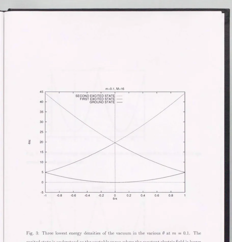
W summarize the results for the vacuum equation below. We show the three lowest energy d nsities in Fig.

3.

The excited states are interpreted as the unstable vacua where the constant electric field 0 is larger than

1r.

W can se it by thinking th massle s case.

In this case the potential is zero and th vacuum equation is th fre equation. The eigenfunction is a plane wave and the eigenvalue is given as 02

/

2. We are now reducing the range of B, and the spectrum out of this region is turned up in the first Brillouin zone.

This is the original form of this 'excited states. For n1a siv ca e, thi al o happen In the same way.

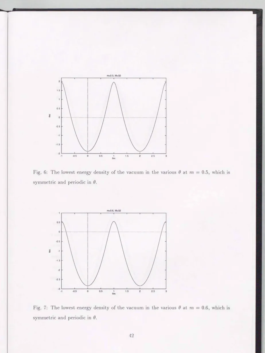
We show the lowest (stable) energy densities of the vacuum for th vanous valu B in the F ig's. 4-9. This is symmetric in B and periodic in the period 21r. The most interesting points in these figures are the behaviors at 0 ₌ 1r. For th strong coupling constant (or the small mass li1nit, where the fern1ion 1nass is now in the unit of th coupling constant

ej ft),

the point at B _{= 1r} is a cusp and not differentiable, but as th fermion mass is increasing, the cusp at () ₌ 1r becomes milder. In th weak coupling the derivative of the vacuum density by B gets equal to zero. This is a kind of the signal of the phase transition at this point. The critical valu is me � 0.5 from these figur s. Th potential term originally comes from the vacuum exp ctation values of th fermionic part of Hamiltonian, therefore the potential is the energy of the Dirac sea. This potential plays such a role as to reduce the energy peak at () _{= 1r} as the fermion mass incrcas s. It is considered as the polarization of the vacuum becom s larger along incr asing the fermion mass.

5 Conclusions and Discussion

We investigate the massive Schwinger 1nodel with great care of the zero Inod of the gauge fields by putting the system into the finite (light-cone) spatial box. After Dirac procedur of quantization for the constrain d system, we regularize the composite operators, the currents and the charge by the point-splitting in gauge invariant way. The chiral anomaly of the axial U(l) current is derived from the anomalous commutation relations of the urrents,

j+

's. Especially the chargcless condition, which is a zero mode of the Gauss law, is derived to be still the first class constraint by using the arbitrariness of the r gularization of the current. Therefore the zero 1node of

A+

is still dynamical degree of fr dom and the chargeless condition is consistently imposed and r lates the

ferrrlion Fock states to the zero mode of th gauge field.

We discuss the residual gaug transfonnation, the large gauge transformation, and by the invariance of the physics under this transfonnation it is derived that th physics is p riodic in B-parameter and symmetric under changing the signs of the background constant electric :field B. This is exactly same as the Bloch Theor m in th olid stat physics in which the system has the symrnetry under the translation of a lattice of the crystal.

We get the signal of the phase transition at B

= 1r

by looking at the energy density of the vacuum. In the strong coupling the vacuum energy density is not differentiable becau it has a cusp. However the cusp becomes gradually milder from the strong coupling to the weak coupling and become differentiable at some critical point.

The physicalrneaning of this phase tran. iLion is a li ttle unclear in our scheme. Colernan says that this is the phase transition of the charge conjugation symmetry [21]. Our r suit is basically consistent with the lattice calculation [34). They looked at the slope of the string tension at B

= 7r.

The string tension is in essence th difference of th en rgy density for B #-

0

and for B

= 0.

They did not include the energy density B2 /2 ^{in the}

strong coupling limit which is correspond d to the massless Schwinger mod 1, then th string tension b comes T( ^B)

⁼

^B2 /2- ⁽

^t:

( B)- t:(O)) in our language, wher

t:

is our vacuum den ity . This value is the same behavior as our results. Th r fore it is justified for us to have found the phase transition at B

= 1r.

We succeeded to look at the phase transition dynan1ically in th light-cone quantization scheme.

In this thesis we ignored the zero mod of the fermions. Even if we take the anti­

periodic boundary condition for the fermions, the dynamical zero mod s of the fermion come arise from the zero point of the Dirac operator of th Eqn. (3.11). How ver it is depend nt on th configuration of the ga.ug field

q. L

t us de:fin th Fourier component of the fern1ions, {; ^Land {;

^R

, respectively. The Eqn. (3.11) becomes as f[(n+1/2)-q]{;L(n)

⁼

h -

^R

( n) and th re is a zero point of the Dirac operator wh n q is a half-int g

r.

In this

case , this constraint becomes

;f;R(n)

^� 0 and

;f;L(n)

r ma1ns a the dynamical d gr e of the freedom only in one value of n. Happily, the Hamiltonian does not involve such a term because its terms always take the fon11s which are the summation of the combination

;f;k(n);f;L(n).

T herefore the vacuum equation does not change basically in this case. It

changes the value of the potential just at the singular point wher the gauge field q is a half-integer. We have solved the singular potential problem with the principal valu prescription and expect that the singularity disappears if we investigate the z ro mode of the left-handed fermion seriously.

Acknowledgments

The author would like to thank our colleagues in Kyushu University, especially Koji Harada and Atsushi Okazaki for a lot of fruitful discussions on this work. H is also gratefu] to Shogo Tanimura (Kyoto Univer ity) and Motoi Tachibana (Kobe Univ rsity), which gave the useful comments to this work.

APPENDIX

A 6-body ^LFTD approximation of QED2

At first we summarize notation and conventions used in this paper. They are ess ntially the same as those by Perry and Harindranath

[10].

The 1netri is given by

wh re

gj.J,V ⁼

(

¹

⁰ ) ^(J-1'

^{1/ =}

^{0' 1)'}

0 -1

g�" ⁼

( : � ) ^(Jl,

^{v = +,}

^-

^),

We treat x+ as our "time". Accordingly, gatnma. matrices are defined as follows;

thus 'ljJ =

('l/JR, 'l/JL)T.

The totally antisymmetric tensor f.J.J-v is defined by

(A.1)

(A.2)

(A.3)

(A.4)

The massive Schwinger model

[20, 21]

is two-di1nensiona.l QED with a massive fermion.

It is not exactly solvable in contrast to th n1assless on [19,

24).

Th Lagrangian is giv n

by

(A.5)

where FIJ-V

=

aJJ-Av-BvAw In two diinensions, the coupling constant

e

has ITiass dimension.

It is therefore useful to measure all dimensionful quantities in units of

e/

.Jii. We her after set

e/ fo

₌

1.

In this unit, strong couplings correspond to small mass s.

In the light-cone gauge

(A+

⁼

0),

only the independent variable is

7/JR

in th light-con quantization.

A-

and

7/JL

are expressed in terms of

7/JR

as follows:

A-

r=

1 ·+

= y7r(i8 _ )21 '

^(A.6)

m

1

7/JL = y'2 i8_ 7/JR., (

A

.7 )

with

j+(x-)

=

v'2: 7/Jk(x-)7/JR(x-)

:. Eliminating A- and

7/JL

by using (A.6) and

(

A.

7 )

, one obtains the light-cone Hamiltonian p-.

(A.S)

We expand

7/JR

in terms of the creation and annihilation operators,

where

b(k+)

and

d(k+)

satisfy the following anti-commutation relations,

(A.lO)

derived from

{7/JR(x-),7/Jk(y-)} = (1/v/2)6(x-- y-).

One may xpress p- entirely in terms of

b(k+)

and

d(k+)

(and their Hermitian conjugates). We refer the reader to Ref.

[5]

for the explicit form.

We work in a truncated Fock space in which a tat with total light-cone mom ntum p+ ⁼ P is expressed as

where we use the abbreviated notations,

b!

=

bt(ki), d!

=

dt(ki)·

In these equations, w rescaled momenta,

ki--+

Xi=

k

i/P and the wave functions,

1/J2(k1, k2), 7/J4(k1, k2; k3, k4),

and

7/J6(ki,k2,k3;k4,ks,k6)

are replaced by

7/J2(x1,x2), p-I'ljJ4(xi,x2;x3,x4),

and

The wave functions

7/J2, 7/J4

and

7/J6

must satisfy the following symmetry properti s due to Fermi statistics,

If we r quir that this state has a definite prop rty under charge conjugation transforma- tion, w have further conditions on these wave functions,

The upper/lower sign in

(A.12)

corresponds to charge conjugation even/odd. This prop­

erty i deriv d by the fact that if

'02(x,

1-

x), 7/J4(x1 x2·

X3,

x4)

and

'l/J6(x1

X2,

x3;

X<�, X5,

x6)

are a solution of the Einstein-Schrodinger equations th n

-�2(1- x, x), �4(x3, x4; x1, x2)

We solve the Einstein-Schrodinger equation:

(A.1 2)

With

(A.11),

we obtain the following coupled integral equations:

(A.13)

4 1

J\/[2�4(x1, x2; x3, x4)

=

(m2- 1)�4(x1, x2; x3, x4) L- ^(A.14)

i=l Xi + Jo r' dy,dy,?j;.(yr, y,; XJ, x.).S(xr + x, -Yr -y,) ( x1 -Y1 1 )' + r' dyr dy,'lj;. ( Xr, x,; Yr, y,).S( XJ + x. -Yr -y,) ( . 1 )'

Jo ^X3-Y1

+4 _Jo {1 dy1dY2�4(x1, Y1; x3, Y2)8(x2 + X4- Y1-Y2) [( � ⁾

^'

^{- ( 1 )}

^'

]

x2 X4 x2 -Y1 +2 Jo {' dy?j;,(y, x4).S(x1 + x2 + x3- y) ( 1 )' x1 -y

-2 e dy?j;,(x,,y).S(xr+x3+x.-y) ( 1 )'

Jo X3-y

-6

Jo (

'

dy,dy,dy37j;6(Yr, y,, x,; y3, X3, x.).S(y, + Y2 + Y3 -x,) ( X1 -Y1 1 )'

+6 Jo {' dy, dy,dy37j;6(Yr, x,, x,; y,, y3, x.).S(y, + y2 + y3 -x3) ( X3- Y2 1 )' ,

6 1

M2'1/J6(x1,x2,x3;x4,x5,x6)

=

(n1-2 -1)'1/J6(xt,X2,x3;x4,x5,x6)L- (A.l5)

i=l Xi

1 ^{1 1}

+3 dy1dY2'1/J6(Y1, Y2, x3; X4, xs, x6)8(x1 + x2-Y1 -Y2) (

o ^{X1 -Y1} )2

+3 lo { I dy1 dy2'if;6( XJ, X2, X3; Yl> Y2, XG)J( X4 + X5 -Y1 -Y2) ( 1 ^{X4-Y1 )2}

+9 ^lo {1 dy1dy2'1/J6(y1, x2, x3; Y2, X5, x6)8(x1 + X4-Y1 -Y2) [( ^{x1 + X4 1 )2 - ( 1 x1 -Y1 )2} ]

-6

lo { 1 dy'if;.(y, x3; X5, x6)0(x1 + x2 + x4-y) ( ^{x1 -y}

1

)2

+6

t dy ,P.(x2,x3;y,x6)0(x1+x•+x5-y)(

¹

)2

lo

^1'4

^-

^y

This is very complicated and one may think too difficult to solv it, but it can b

converted to a single matrix eigenvalue quation by expanding the wave functions in terms of basis functions. The basis functions are decided according to its symmetries above and its behavior at

x

^{= 0}

,1

. It is well known that the wave function

'l/J2(x,1-x)

behaves as

xf3

in the vicinity of

x

^{= 0}

[4],

with {3 b ing the solution of th equation

m2 -

1

+

n{3cot

(

^n{3

)

^{= 0.} By taking it into account, Mo and Perry concluded that

a useful choice of the basis functions for the wave functions is given in terms of Jacobi polynomials,

p�/3,/3).

In a previous paper

[

^6,

^7],

we propose a simpler s t of basis functions, essentially equivalent to that of Mo and Perry. For example

'lj;2( x,

1

-x)

is decomposed by polynomials

[x(1-x)]f3+k

and

[x(1-x)]f3+k (2x-

1), where k is integ r. In th 2- body, the charge conjugation is defined by x H 1

-x,

th y correspond to the charge conjugation odd and even, resp ctively due to F rmi statistics. For the explicit form of the basi function for the 4-body and 6-body wave functions, see Refs.

[7].

It is important that we can obtain the matrix element analytically by using thes basis functions. We now get a simple matrix equation, then we diagonalize it and obtain the eigenvalues and eig nfunctions with the computer.

B "Iterative property" of Dirac brackets

In the light-cone quantization, one usually face with a lot of constraint . It is sometim s very tedious to calculate Dirac brackets directly. In this app ndix we explain the "iterative method"

[30)

of calculating Dirac brackets for the r adcrs who are not familiar with it.

The most tedious part of the calculation is to g t the inverse of the constraint matrix CIJ

=

{OI,BJ}, where 81,

(I= 1,

^{· · ·}

,2N)

are the second-class constraints of the th ory.

(For simplicity, we assume that there is no first-class constraints. The generaUzation to such cases with first-class constraints is trivial.) We divide these constraints into two groups, for example: B1

= ((/Yi, c.pj),

where 1

::; i::; 2m, 1 ::; j::; 2N- 2m

for arbitrary

m (1 ^::;

Tn <

N).

We denote this constraint n1atrix as follows:

c

= ( { c/Y, cP}

{c.p,c/Y}

{ c/Y, c.p} )

⁼

(

^{X Z}

)

^'

{ c.p' c.p}

^{- zr y}

where we introduce the abbreviations X, Y _and Z. What we want to do is to calculate th inverse of C in (more than) two steps. First we calculate the 'Dirac brackets' constrained on the surfac

cPi

^�

0

Let us call thes brackets "D 1 brackets." We have to calculate "D1 brackets" for all the

variable. and set

cPi

strongly equal to zero. Note that the constraint matrix for the rest

'Pj

changes because of this procedure, namely,

!11ij

⁼

{c.pi,'Pj}Dl

⁼

{c.pi,'Pj}- {c.pi,cPk}(x-l)k1{c/Yt,c.pj},

M = Y + zrx-1Z.

(B.1)

The iterative property is the property that the correct Dirac bracket for physical variables F _and G is obtained in the following way:

namely, we can calculate the Dirac brackets in two t p . Obviously w can g neraliz the above procedure to many step calculations.

The proof is quite simple. In terms of Poisson brack t , the Dirac bracket

(B.2) ¹

s given as follows:

{F,G}n

=

{F,G}- {F,4>i}(X-1)ij{4>j,G}

where

n

is given by

+

{F, cPk}(X-1 )kl Zti(M-1 )ij Zjm(X-1 )mn{ 4>n, G}

+

{F,4>k}(X-1)ktzti(M-1)ij{<pj,G}

- { F, <pi}(M-1 )ij Zjk(x-1 )kt { 4>t, G}

- {F,<pi}(M-1)ij{<pj,G}

=

{F, G}- {F,

lh

}nu {OJ, G},

( x-1- x-1zM-1zrx-1

fl=

M-1 zr x-1

One can easily see that

n

is the inverse of C.

C Currents and anomaly

(B.3)

(B.4)

(B.5)

In this app ndix, we discuss the regularization of the current, the Schwiger term, and chiral anomaly. In order to have a well-defined quantum theory, one must regularize th current properly so that it repro duces the well-known chiral anomaly.

The massive Schwinger model is a gauge invariant theory. One should pres rve gauge invariance in any regularization. Actually it is possible. On the oth r hand, axial symme­

try is broken anomalously at the quantu1n level. There is no consistent way to preserve both symmetri s.

Let us begin with our Fourier expansion of the fermion field

(3.22).

By substituting

it into th gauge invariant definition of the ^CUlT nt (3.24), we get

j+(x)

⁼

^,j2: .J;k1/JR(x)

^{:N +2}

�

^(N-

^q),

j-(x)

⁼

^V2: ?fitV;L(x)

^:N

-;-A-

_21r

(C.1) (C.2)

1n our gaug condition. The normal-ordering is with respect to the N-vacua. See Eqn. (3.26). In deriving these, we used the following properties[4],

(C.3) (C.4)

As explained in the text, we think that the zero mode (the charge) has nothing to do with th non-zero modes and "adjust" the zero mode so that it satisfi s desired properti s.

InS c. 3.2, we have constructed such a charge. We only require that the nonzero mod s of the vector and axial vector currents satisfy the conservation and anomalous conservation laws respectively.

In order to calculate the divergences of the currents, we need the commutator of the current,

[J+(x),)+(y)].

By a straightforward calculation, we get

(C.5)

where the sums do not converge. We make them convergent by adding (or subtracting) a small imaginary part in the exponents. We get

--:+ --:+ -

1 . 1 1

[J (x),J (y)]-

-4 7r

ll

f-r

po[(

X

- y

+ ^{Zf. .}

)2

₍ ^X -

y -

^zt . )2]

= _z

S'(x- y)

+

O(L-2).

27r (C.6)

In this way, we can reproduce the correct Schwinger term in the "continuum" limit.

It is now easy to calculate the current diverg nces. By using th anomalou commu- tation relation ( C.6), _{one get}

The spatial derivative of ] _- (

_x

) _is

(C.8)

From these we get the divergences of the vector current and the axial vector current:

(C.9)

(C.lO)

where we use the relation

1J.L15

= -

_{EJ.Lv ft/)}

(

_{E+- =}

_-1).

How about the axial charge? As explain d in the text, it is formally equal to the (vector) charge. But because the axial vector current is not conserved, we expect that the axial charge is

not

conserved. In conclusion, there is no such a charge on the light-cone.

Remen1ber that the left-handed field '1/JL is not an independent fi ld. The independent fields are 'lfJR and

0 A-.

It is well-known that axial-vector transformations are inconsistent

on the light cone[35], i.e., they are inconsistent with the constraint quation (3.11). What if one wants to define the axial-vector transfonnations only for the independent field

'lfJ R ? Because of !s'l/JR = _{'1/J R} it is equivalent to the usual (v ctor) phase transformations.

One cannot define an axial-vector transformation, different from the usual (vector) phase transformation, in a self-consistent way. It means that the axial charge, which is suppos d to be the g n rator of the transformation do s not exit.

M ustaki proposed another definition of the axial- vector current which is cons rved

even for massive

f

rmions[35]. Does it lead us to another definition of axial charge?

Unfortunat ly it does not. Mustaki's cons rved current is nothing but the v ctor current

in the rnassive Schwinger model.

References

[1) R. J. Perry, A. Harindranath, and K. G. Wilson, Phys. R v. L tt. 65, 2959 (1990).

An extensive list of references on light-front physics by A. Harindranath (light.t x) i available via anony mous ftp from public.mps.ohio-state.edu und r the subdir ctory tmp/infolight.

[2) K. G. Wilson, T. S. Walhout, A. Harindranath, W. M. Zhang, R. J. Perry, and S .D.

Glazek, Phy . Rev D49, 6720 (1994).

[3) S. J. Brodsky, G. McCartor, H. C. Pauli and S. S. Pinsky, Particle World 3, 109 (1993).

[4) H. Bergknoff, Nucl.Phys. B122, 215 (1977) .

[5) Y. Mo and R. J. Perry, J. Comp. Phys. 108, 159 (1993).

[6) K. Harada, M. Sugihara, M. Taniguchi, M. Yahiro, Phys. Rev. D49, 4226 (1994).

[7) K. Harada, A. Okazaki, and M. Taniguchi, Phys. Rev. D52, 2429 (1995) [8) K. Harada, A. Okazaki, and M. Taniguchi, preprint, KYUSHU-HET-28.

[9) T. Sugihara, M. Matsuzaki, and M. Yahiro, Phys. Rev. D50,5274 (1994).

[10) R. J. Perry and A. Harindranath, Phys. Rev. D43, 4051 (1991 ).

[11) K. Hornbostel, S. J. Brodsky, and H. C. Pauli, Phys. Rev. D41, 3814 (1990); S. Dal­

ley, I. R. Klebanov, Phys. Rev. D47, 2517 (1993); Phys. Lett. B298 79 (1993); G.

Bhanot, K. Demeterfi, and I. R. Klebanov, Phys. Rev. D48 4980 (1993). K. Deme­

ter£., I. R. Klebanov, and G. Bhanot, Nucl. Phys. B418 15 (1994); Y. Matsumura, N. Sakai, and T. Sakai, Phys. Rev. D52, 2446 (1995)

[12) H. C. Pauli and S. Brodsky, Phys. Rev. D32, 1993 (1985); 32, 2001 (1985); T. Ell r, H. C. Pauli, and S. Brodsky, Phys. Rev. D35 1493 (1987);