complex space forms

A characterization of ruled hypersurfaces and homogeneous real hypersurfaces of type (A

), (A

), and (B) in non-flat

complex space forms

Setsuo Nagai

Dedicated to Professor U-Hang Ki and Professor Masafumi Okumura on the occasion of their 80th birthdays

Abstract. The purpose of this paper is to give a characterization of ruled hypersurfaces and homogeneous real hypersurfaces of type (A

), (A

), and (B) in non-flat complex space forms by using the second covariant derivatives of the shape operators.

1. Introduction

Let M

(c) be an n-dimensional complex space form with constant holo- morphic sectional curvature c ̸ = 0, and let J and g be its complex structure and K¨ ahler metric, respectively. Complete and simply connected complex space forms are isometric to either a complex projective space C P

(c) or a complex hyperbolic space CH

(c) decided from c > 0 or c < 0, respectively.

Let M be a connected submanifold of M

(c) with real codimension 1.

We refer to this simply as a real hypersurface below. The induced metric of M is denoted by g. For a local unit normal vector field ν of M , we define the structure vector ξ of M by ξ = − J ν. Further, the structure tensor field ϕ is defined by J X = ϕX + g(X, ξ)ν . The structure vector ξ is said to be

2010 Mathematics Subject Classification. Primary 53B25; Seondary 53C15.

Key words and phrases. homogeneous real hypersurface, ruled hypersurface, complex space form.

115

principal if Aξ = αξ is satisfied for some function α, where A is the shape operator of M .

A real hypersurface M is said to be a Hopf hypersurface if the structure vector ξ of M is principal. In a complex projective space C P

(c), Hopf hy- persurfaces with constant principal curvatures are simply the homogeneous real hypersurfaces (for details, see §2 Theorem K). They were classified by R. Takagi [14] (for details, see § 2 Theorem T), and their principal cur- vatures were also calculated by R. Takagi [15] (for details, see § 2). In a complex hyperbolic space C H

(c), Hopf hypersurfaces with constant prin- cipal curvatures were classified by J. Berndt [2] (for details, see § 2 Theorem B).

On the other hand, there are important examples of non-Hopf hypersur- faces in M

(c), such as ruled hypersurfaces (for definition, see § 2), with a totally geodesic ruling along a curve in M

(c).

For a real hypersurface M in M

(c), let T

be a distribution defined by T

= {X ∈ T M| g(X, ξ ) = 0}, where T M denotes the tangent bundle of M. The distribution T

is called a holomorphic distribution (see [9]). T

is not integrable on any Hopf homogeneous real hypersurface of M

(c) but is integrable on any ruled hypersurface of M

(c). M. Kimura [5] obtained some properties of a ruled hypersurface of C P

(c) and gave an example of minimal ruled hypersurface of C P

(c). There are many characterization theorems of ruled hypersurfaces in M

(c) (e.g., [1], [4], [6], [7], [9]). We also know many characterization theorems of homogeneous real hypersur- faces by using some formulas of the first covariant derivatives of the shape operators (e.g., [3], [7], [8], [9]).

In [12], we characterized homogeneous real hypersurfaces of type (A

) and (B ) simultaneously by using the second covariant derivatives of the shape operators under the conditions that the structure vector fields ξ are principal as follows:

Theorem N.[12][Theorem 4.1.] Let M be a connected real hypersurface in

a complex space form M

(c) (n ≥ 2, c ̸ = 0) on which the structure vector

ξ is principal with principal curvature α ̸ = 0. Then the shape operator A

satisfies

g(( ∇

A)Z, W ) = α 4

{

g(ϕAX, Y )g((4ϕA + 2c

α ϕ)Z, W ) + g(ϕAX, Z)g((4ϕA + c

α ϕ)Y, W ) +g(ϕAX, W )g((4ϕA + c

α ϕ)Y, Z) }

, X, Y, Z, W ∈ T

,

if and only if M is locally congruent to a homogeneous real hypersurface of type (A

) or (B).

The purpose of this paper is to generalize the above result. To that end, we prove the following theorem:

Theorem 4.1. Let M be a connected real hypersurface in a complex space form M

(c) (n ≥ 3, c ̸ = 0). Then the shape operator A satisfies the following equation for some nonzero constant a:

g((∇

A)Z, W ) = c

4a {2g(ϕAX, Y )g((2ϕA + aϕ)Z, W ) + g(ϕAX, Z)g((4ϕA + aϕ)Y, W ) +g(ϕAX, W )g((4ϕA + aϕ)Y, Z) } , X, Y, Z, W ∈ T

,

(4.1)

if and only if M is locally congruent to one of the following:

(A

) a horosphere in C H

(c);

(A

) a geodesic hypersphere in M

(c) or a tube over a complex hyperbolic hyperplane C H

(c) in C H

(c);

(B) a tube over a totally geodesic and totally real space form of real di- mension n in M

(c);

(R) a ruled hypersurface in M

(c).

In the following all manifolds are assumed to be C

and connected.

2. Preliminaries

In this section, we present some preliminary results of real hypersurfaces in a complex space form.

Let M

(c) (c ̸ = 0) be an n-dimensional complex space form with constant holomorphic sectional curvature c and let J and g be its complex structure and K¨ ahler metric, respectively.

M is a real hypersurface of M

(c). Further, we denote by g the induced Riemannian metric on M and by ν a local unit normal vector field along M in M

(c).

The Gauss and Weingarten formulas are:

∇

Y = ∇

Y + g(AX, Y )ν, (2.1)

∇

ν = − AX, (2.2)

where ∇ and ∇ respectively denote the Levi–Civita connection on M

(c) and M , and A is the shape operator of M in M

(c).

We define an almost contact metric structure (ϕ, ξ, η, g) on M as in the usual way:

ξ = − J ν, η(X) = g(X, ξ), ϕX = (J X)

, X ∈ T M, (2.3) where ( )

denotes the tangential component of a vector. These structure tensors satisfy the following equations:

ϕ

= − I + η ⊗ ξ, ϕξ = 0, η ◦ ϕ = 0, η(ξ) = 1, (2.4) where I denotes the identity mapping of T M.

From (2.1) and (2.3), we easily have

( ∇

ϕ)Y = η(Y )AX − g(AX, Y )ξ, (2.5)

∇

ξ = ϕAX, (2.6)

for tangent vectors X, Y ∈ T M.

In our case the Gauss and Codazzi equations of M become R(X, Y )Z = c

4 { g(Y, Z)X − g(X, Z )Y + g(ϕY, Z)ϕX

− g(ϕX, Z )ϕY − 2g(ϕX, Y )ϕZ } + g(AY, Z)AX − g(AX, Z)AY,

(2.7)

( ∇

A)Y − ( ∇

A)X = c

4 { η(X)ϕY − η(Y )ϕX − 2g(ϕX, Y )ξ } . (2.8) The Ricci formula of the tensor field T on M is:

∇

T − ∇

T = R(X, Y ) · T, X, Y ∈ T M, (2.9) where the second covariant derivative ∇

T of T is defined by

∇

T = ∇

( ∇

T ) − ∇

T and R(X, Y ) acts on T as a derivation.

A real hypersurface M of CP

(c) is said to be a homogeneous real hy- persurface if it is an orbit of an analytic subgroup of the isometry group of C P

(c). We know the complete classification of homogeneous real hyper- surfaces of C P

(c).

Theorem T ([14]). Let M be a homogeneous real hypersurface of C P

(c).

Then M is locally congruent to one of the following spaces:

(A

) a geodesic hypersphere;

(A

) a tube of radius r (0 < r <

c

) over a totally geodesic C P

(c) (1 ≤ k ≤ n − 2);

(B) a tube of radius r (0 < r <

) over a complex quadric Q

; (C) a tube of radius r (0 < r <

c

) over C P

× C P

2

where n ( ≥ 5) is odd;

(D) a tube of radius r (0 < r <

c

) over a complex Grassmann G

and n = 9;

(E) a tube of radius r (0 < r <

) over a Hermitian symmetric space SO(10)/U (5) and n = 15.

For homogeneity of a real hypersurface in CP

(c), there is a criterion obtained by M. Kimura [5]. His theorem is

Theorem K ([5]). Let M be a connected real hypersurface in C P

(c).

Then M has constant principal curvatures and the structure vector ξ is

principal if and only if M is congruent to an open subset of a homogeneous real hypersurface.

In CH

(c) J. Berndt [2] obtained the complete classification of Hopf hypersurfaces with constant principal curvatures. His theorem is the fol- lowing:

Theorem B ([2]). Let M be a connected real hypersurface of CH

(c) (n ≥ 2) with constant principal curvatures. Further, assume that the structure vector ξ is principal. Then M is orientable and holomorphic congruent to an open part of one of the following hypersurfaces:

(A

) a horosphere in C H

(c);

(A

) a geodesic hypersphere or a tube over a complex hyperbolic hyperplane CH

(c) in CH

(c);

(A

) a tube of radius r ∈ R

over a totally geodesic C H

(c) (1 ≤ k ≤ n − 2);

(B) a tube of radius r ∈ R

over a totally geodesic totally real submanifold RH

.

Concerning the principal curvatures α, λ

, λ

, λ

, λ

and their mul- tiplicities m

, m

, m

, m

, m

of homogeneous real hypersurfaces in CP

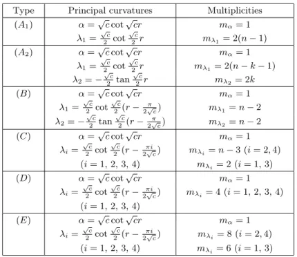
(c), we have the following Table 1 (see [15]): Here, α is the principal curvature corresponding to the principal direction ξ.

Concerning the principal curvatures α, λ

, λ

and their multiplicities m

, m

, m

of Hopf homogeneous real hypersurfaces in C H

(c), we have the following Table 2 (see [10]): Here, α is the principal curvature corresponding to the principal direction ξ.

Next, we explain some fundamental facts of ruled hypersurfaces in com- plex space forms (for details, see [1], [4], [5], [6]). Let γ : I → M

(c) be an arbitrary (regular) curve in M

(c). Then for every t ( ∈ I) there exists a totally geodesic hyperplane M

(c) (in M

(c)) through the point γ(t) which is orthogonal to the holomorphic plane spanned by γ

(t) and J γ

(t).

Let M = ∪

t∈I

M

(c). Then M obtains a real hypersurface of M

(c),

which is called a ruled hypersurface.

Type Principal curvatures Multiplicities

(A

) α = √

c cot √

cr m

= 1

λ

=

cot

r m

= 2(n − 1)

(A

) α = √

c cot √

cr m

= 1

λ

=

cot

r m

= 2(n − k − 1) λ

= −

tan

r m

= 2k

(B) α = √

c cot √

cr m

= 1

λ

=

cot

(r −

) m

= n − 2 λ

= −

tan

(r −

) m

= n − 2

(C) α = √

c cot √

cr m

= 1

λ

=

cot

(r −

) m

= n − 3 (i = 2, 4) (i = 1, 2, 3, 4) m

= 2 (i = 1, 3)

(D) α = √

c cot √

cr m

= 1

λ

=

cot

(r −

) m

= 4 (i = 1, 2, 3, 4) (i = 1, 2, 3, 4)

(E) α = √

c cot √

cr m

= 1

λ

=

cot

(r −

) m

= 8 (i = 2, 4) (i = 1, 2, 3, 4) m

= 6 (i = 1, 3)

Table 1: Principal curvatures in C P

(c)

Type Principal curvatures Multipricities

(A

) α = √

− c 1

λ

=

2n − 2

(A) α = √

− c coth √

− cr 1 λ

=

coth

r 2(n − k − 1) λ

=

tanh

r 2k

(B) α = √

− c tanh √

− cr 1 λ

=

coth

r n − 1 λ

=

tanh

r n − 1

Table 2: Principal curvatures in C H

(c)

Let T

= { X ∈ T M | X ⊥ ξ } be the holomorphic distribution of M.

Then the distribution T

is integrable on a ruled hypersurface M . Fur-

thermore, the shape operator A of M satisfies the following:

Aξ = αξ + U (U ̸ = 0), AU = g(U, U)ξ,

AX = 0, X ⊥ ξ, U,

(2.10)

where U is the T

-component of Aξ (for details, see [6]).

Now, we define the concept of η-parallel second fundamental form as follows.

Definition 2.1. The shape operator A of a real hypersurface M is said to be η-parallel if A satisfies the following:

g(( ∇

A)Y, Z) = 0, X, Y, Z ∈ T

. (2.11)

There are many characterization theorems for ruled hypersurfaces in a complex space form (see, for example, [1], [4], [5], [6], [7]). The following proposition can be easily deduced:

Proposition 2.2. Let M be a real hypersurface of a complex space form M

(c). If the shape operator A of M satisfies

g(AX, Y ) = 0, X, Y ∈ T

, (2.12) then M is locally congruent to a ruled hypersurface of M

(c).

Proof Let X and Y be vector fields of M whose values belong to T

. Then, accoding to (2.6) and (2.12), we have

g( ∇

Y, ξ) = − g(Y, ϕAX) = g(AX, ϕY ) = 0.

This means that

∇

Y ∈ T

, X, Y ∈ T

. (2.13) Furthermore, for vector fields X and Y whose values belong to T

, we have

∇

Y = ∇

Y + g(AX, Y )ν = ∇

Y. (2.14)

From (2.13) and (2.14), we conclude that the leaves of the distribution T

are totally geodesic in M and in M

(c). Because T

is J -invariant, all

the leaves of the distribution T

are totally geodesic complex hyperplanes

M

(c) of M

(c). This proves the proposition.

Remark 2.3. For a real hypersurface M of M

(c), the following two con- ditions are equivalent (see Proposition 5 in [7]):

(i) The holomorphic distribution T

is integrable.

(ii) g((ϕA + Aϕ)X, Y ) = 0 for any X, Y ∈ T

.

Remark 2.4. Under the condition of Proposition 2.2, the shape operator A of M is η-parallel (see [7] Proposition 4).

For ruled real hypersurfaces in a complex space form, M. Kimura and S. Maeda obtained the following characterization theorem:

Theorem 2.5 (M. Kimura and S. Maeda [7]) Let M be a real hyper- surface of C P

(c). Then the shape operator A of M is η-parallel and the holomorphic distribution T

is integrable if and only if M is locally congru- ent to a ruled hypersurface of C P

(c).

For a ruled hypersurface of M

(c), S-S. Ahn, S-B. Lee, and Y-J. Suh ob- tained the following:

Theorem 2.6 (S-S. Ahn, S-B. Lee, and Y-J. Suh [1]) Let M be a con- nected real hypersurface of M

(c), c ̸ = 0 and n ≥ 3. If the shape operator A of M satisfies

g(( ∇

A)Y, Z) = 0 and

g((Aϕ − ϕA)X, Y ) = 0

for any vector fields X, Y , and Z in T

, and the structure vector field ξ is not principal, then M is locally congruent to a ruled hypersurface.

3. Lemmas

In this section, we present some lemmas that we will use to prove our main theorem.

For the shape operators of real hypersurfaces in a non-flat complex space

form M

(c) (c ̸ = 0), we know the following:

Lemma 3.1 ([11], [13]) Let M be a homogeneous real hypersurface of type (A) in a non-flat complex space form M

(c) (c ̸ = 0). Then the shape operator A of M satisfies the following equations:

ϕA − Aϕ = 0, (3.1)

A

− αA − c

4 I = − c

4 η ⊗ ξ, (3.2)

( ∇

A)Y = − c

4 { η(Y )ϕX + g(ϕX, Y )ξ } , (3.3) where α and I denote the principal curvature in the direction of the structure vector ξ and the identity mapping of T M, respectively.

Lemma 3.2 ([3]) Let M be a homogeneous real hypersurface of type (A

) or (B) in a non-flat complex space form M

(c) (c ̸ = 0). Then the shape operator A of M satisfies the following equations:

ϕA + Aϕ + c

α ϕ = 0, (3.4)

A

+ c α A − c

4 I = (α

+ 3

4 c)η ⊗ ξ, (3.5)

( ∇

A)Y = − α

4 { 2η(X)(Aϕ − ϕA)Y

+η(Y )(Aϕ − 3ϕA)X + g((Aϕ − 3ϕA)X, Y )ξ } .

(3.6)

From Lemma 3.1, Lemma 3.2, Table 1 and Table 2, we have

Lemma 3.3. Let M be a homogeneous real hypersurface of type (A

), (A

), or (B) in M

(c) (c ̸ = 0). Then, the shape operator A of M satisfies the following equations for some nonzero constant a:

ϕA + Aϕ + aϕ = 0, (3.7)

( ∇

A)Y = c

4a { 2η(X)(2ϕA + aϕ)Y + η(Y )(4ϕA + aϕ)X +g((4ϕA + aϕ)X, Y )ξ} .

(3.8)

So, taking the covariant derivative of (3.8), we have the following:

Lemma 3.4. Let M be a homogeneous real hypersurface of type (A

), (A

), or (B) in M

(c) (c ̸ = 0). Then, the shape operator A of M satisfies the following equation for some nonzero constant a:

g((∇

A)Z, W ) = c

4a {2g(ϕAX, Y )g((2ϕA + aϕ)Z, W ) + g(ϕAX, Z)g((4ϕA + aϕ)Y, W )

+g(ϕAX, W )g((4ϕA + aϕ)Y, Z) } , X, Y, Z, W ∈ T

. (3.9) For a ruled hypersurface in M

(c) (c ̸ = 0), we have

Lemma 3.5. Let M be a ruled hypersurface in M

(c) (c ̸ = 0). Then, both-sides of (3.9) vanish.

Proof For a ruled hypersurface M , the leaves of the distribution T

are totally geodesic both in M and M

(c). Furthermore, the shape operator A of M is η-parallel (see [6]). From this it follows that

g(( ∇

A)Z, W )

=g( ∇

(( ∇

A)Z) − ( ∇

A)( ∇

Z), W ) − g(( ∇

A)Z, W )

=0, X, Y, Z, W ∈ T

.

This means that the left side of (3.9) vanishes.

According to (2.10) and Remark 2.3, the right side of (3.9) also vanishes.

This proves the lemma.

The following is known about the principal curvatures of a Hopf hyper- surface:

Lemma 3.6 ([8], [13]) Let M be a Hopf hypersurface of M

(c) (n ≥ 2, c ̸ = 0). Then the principal curvature α corresponding to the structure vector ξ is locally constant, and for any principal curvature vector X ∈ T

with AX = λX , we have

(2λ − α)AϕX = (αλ + c

2 )ϕX.

4. Proof of Theorem

In this section we shall prove our main theorem.

Theorem 4.1. Let M be a connected real hypersurface in a complex space form M

(c) (n ≥ 3, c ̸ = 0). Then the shape operator A satisfies the following equation for some nonzero constant a:

g(( ∇

A)Z, W ) = c

4a { 2g(ϕAX, Y )g((2ϕA + aϕ)Z, W ) + g(ϕAX, Z)g((4ϕA + aϕ)Y, W ) +g(ϕAX, W )g((4ϕA + aϕ)Y, Z) } , X, Y, Z, W ∈ T

,

(4.1)

if and only if M is locally congruent to one of the following:

(A

) a horosphere in C H

(c);

(A

) a geodesic hypersphere in M

(c) or a tube over a complex hyperbolic hyperplane C H

(c) in C H

(c);

(B) a tube over a totally geodesic and totally real space form of real di- mension n in M

(c);

(R) a ruled hypersurface in M

(c).

By making use of the Codazzi equation (2.8), we find the following general formula:

g((∇

A)Z − (∇

A)Y, W )

= c

4 { g(ϕAX, Y )g(ϕZ, W ) − g(ϕAX, Z)g(ϕY, W )

− 2g(ϕAX, W )g(ϕY, Z) } ,

(4.2)

on arbitrary tangent vectors X, Y , Z, W ∈ T

. Therefore the condition (4.1) and (4.2) implies that

g(ϕAX, W )g((ϕA + Aϕ + aϕ)Y, Z) = 0. (4.3)

We assume here that a ̸ = 0.

In what follows e

, . . . , e

denotes an orthonormal basis of T

at a point in M , and the index j runs from 1 to 2n − 2. Letting X = e

and W = ϕe

in (4.3), and taking the summation on j, we have

(h − α)g((ϕA + Aϕ + aϕ)Y, Z) = 0, (4.4) where h and α denote the mean curvature of M and the function defined by α = g(Aξ, ξ), respectively. Furthermore, letting Y = e

and Z = ϕe

in (4.4) and taking the summation on j, we obtain

(h − α) { (h − α) + (n − 1)a } = 0. (4.5) From (4.5) either h − α = 0 or (h − α) + (n − 1)a = 0 holds on M , since M is connected and a ̸ = 0. We therefore devide the discussion into the following two cases:

Case 1. The equation h − α = 0 holds on M .

Case 2. The equation (h − α) + (n − 1)a = 0 holds on M .

We first consider Case 1, in which we have (h − α)+(n − 1)a = (n − 1)a ̸ = 0.

So, from (4.3), the following holds on M :

g(ϕAX, Y ) = 0, X, Y ∈ T

. (4.6) This leads to

Aξ = αξ + U, AU = g(U, U )ξ, AX = 0, X ⊥ ξ, U,

where the vector field U is defined by U = Aξ − αξ. This means that M is locally congruent to a ruled hypersurface of M

(c) by Proposition 2.2 (see also [7]).

On the other hand, let M be a ruled hypersurface of M

(c). Then, (4.1) holds by Lemma 3.5.

We next consider Case 2. In this case we have h − α ̸ = 0. So, from (4.4),

(ϕA + Aϕ + aϕ)X = − g(ϕU, X)ξ, X ∈ T

. (4.7)

On the other hand, using (4.1), (2.7), and (2.9), we have c

4 { g((ϕA + Aϕ)Y, Z)g(ϕX, W ) − g((ϕA + Aϕ)X, Z )g(ϕY, W ) + g((ϕA + Aϕ)Y, W )g(ϕX, Z ) − g((ϕA + Aϕ)X, W)g(ϕY, Z) }

− c

2 { g((ϕA − Aϕ)Z, W )g(ϕX, Y ) + g((ϕA + Aϕ)X, Y )g(ϕZ, W ) }

− c

a g((ϕA + Aϕ)X, Y )g(ϕAZ, W ) + g(AY, Z )g( c

4 X − A

X, W )

− g(AX, Z)g( c

4 Y − A

Y, W ) − g(AX, W )g( c

4 Y − A

Y, Z) + g(AY, W )g( c

4 X − A

X, Z ) = 0, X, Y, Z, W ∈ T

(4.8)

(for details, see [12]).

Combining (4.7) with (4.8), we are led to g(AY, Z )g( c

4 X − A

X, W ) − g(AX, Z)g( c

4 Y − A

Y, W )

− g(AX, W )g( c

4 Y − A

Y, Z) + g(AY, W )g( c

4 X − A

X, Z ) = 0.

(4.9)

We assert that ξ is principal. We shall prove our assertion by reductio ad absurdum.

Let Ω be the open subset of M defined by Ω = { p ∈ M | U (p) ̸ = 0 } . In the following we assume that the set Ω is not empty and all discussion concerns the set Ω unless otherwise stated.

We restate the orthonormal frame field e

, e

, . . ., e

in such a way that e

= ξ, e

= U/ ∥ U ∥ , e

= ϕe

, e

= ϕe

(i ≥ 2).

We now define the local differentiable functions α, β, γ, δ, and h

as follows:

α = g(Aξ, ξ), β = g(Aξ, e

), γ = g(Ae

, e

), δ = g(Ae

, e

), h

= g(Ae

, e

), i, j = 1, 2, . . . , 2n − 1.

Hereafter the index p runs 2, 4, . . ., 2(n − 1) and p ∗ means p ∗ = p + 1. We further assume that e

(i ≥ 4) are chosen in such a manner that

h

= λ

δ

. (i, j ≥ 4).

This is in fact possible by (4.7). Furthermore, the following are satisfied by (4.7):

g(Ae

, e

) = − (γ + a), λ

= − (λ

+ a), p = 4, 6, . . . , 2(n − 1).

Let us first demonstrate the following lemma:

Lemma 4.2. h

= h

= 0 (p = 4, 6, . . . , 2(n − 1)).

Proof Letting X = e

, Y = ϕe

, Z = e

, W = e

in (4.9), we have

− δ(λ

+ a)h

+

{

γ(λ

− a) − β

− 2γ

− 2δ

− ∑

p

h

− ∑

p

h

+ c 4

} h

= 0.

(4.10)

Letting X = e

, Y = ϕe

, Z = e

, W = ϕe

in (4.9), we have δλ

h

+ {

2δ

+ 2(γ + a)

+ ∑

p

h

+ ∑

p

h

− c

4 − (γ + a)(λ

+ 2a) }

h

= 0.

(4.11) Letting X = e

, Y = ϕe

, Z = e

, W = e

in (4.9), we have

{

γ (λ

+ 2a) + β

+ 2γ

+ 2δ

+ ∑

p

h

+ ∑

p

h

− c 4

} h

+ δλ

h

= 0.

(4.12)

Letting X = e

, Y = ϕe

, Z = e

, W = ϕe

in (4.9), we have {

(γ + a)(λ

− a) + 2δ

+ 2(γ + a)

+ ∑

p

h

+ ∑

p

h

− c 4

} h

+ δ(λ

+ a)h

= 0.

(4.13)

From (4.10) and (4.11), we have aδh

+ {

a(λ

− γ) + β

}

h

= 0. (4.14) From (4.12) and (4.13), we have

{ a(λ

+ γ + a) − β

}

h

+ aδh

= 0. (4.15)

Letting X = e

, Y = e

, Z = e

, W = ϕe

in (4.9), we have

{δh

+ (λ

− γ )h

} h

= 0. (4.16) Letting X = ϕe

, Y = e

, Z = e

, W = e

in (4.9), we have

{ (λ

+ γ + a)h

+ δh

} h

= 0. (4.17) From (4.15) and (4.17),

β

h

= 0, and from (4.14) and (4.16),

β

h

= 0.

Since β ̸ = 0, the lemma holds.

Secondly, we prove the following lemma:

Lemma 4.3. δ = 0.

Proof We shall prove the lemma by reductio ad absurdum. We assume that δ ̸ = 0 is satisfied. Then, letting X = e

, Y = e

, Z = e

, W = ϕe

in (4.9) and using Lemma 4.2, we are led to

λ

+ aλ

− c

4 = 0. (4.18)

This leads to λ

̸ = 0 since c ̸ = 0. Letting X = e

, Y = e

, Z = e

, W = e

in (4.9), we have

γ(λ

− c

4 ) − (β

+ γ

+ δ

)λ

= 0. (4.19) Combining (4.18) with (4.19), we have

aγ + β

+ γ

+ δ

= 0. (4.20) Letting X = ϕe

, Y = e

, Z = e

, W = ϕe

in (4.9), we have

(γ + a)(λ

− c 4 ) + λ

{

δ

+ (γ + a)

− c 4

}

= 0. (4.21)

Combining (4.18) with (4.21), we have δ

+ (γ

+ aγ − c

4 ) = 0. (4.22)

Letting X = e

, Y = e

, Z = e

, W = ϕe

in (4.9), we have (γ + a)

{

(λ

+ a)

− c 4

} − (λ

+ a) {

δ

+ (γ + a)

− c 4

}

= 0. (4.23) Combining (4.18) with (4.23), we have

{ γ (γ + a) + δ

}

λ

+ a(δ

+ γ

+ aγ − c

4 ) = 0. (4.24) From (4.22), (4.24), and λ

̸ = 0, we are led to

c = 0,

which is a contradiction, so δ = 0 must be satisfied.

Thirdly, we establish the following lemma:

Lemma 4.4.

λ

= λ

= − a

2 , γ = −( c 2a + a).

Proof Letting X = e

, Y = ϕe

, Z = ϕe

, W = e

in (4.9) and using Lemma 4.2 and Lemma 4.3, we have

(γ + a)β

+ (2γ + a)(γ

+ aγ − c

4 ) = 0. (4.25) Equation (4.21) is reduced to

(λ

+ γ + a) {

λ

(γ + a) − c 4

}

= 0. (4.26)

Also, (4.23) is reduced to (λ

− γ)

{

(λ

+ a)(γ + a) + c 4

}

= 0. (4.27)

Letting X = e

, Y = e

, Z = e

, W = e

in (4.9), we have (2λ

+ a)(λ

+ aλ

− c

4 ) = 0. (4.28)

We assert that λ

̸= γ. If λ

= γ were satisfied, we would have (γ +a)β

= 0 from (4.25) and (4.28). Since β ̸ = 0, we further would have γ = − a. Then, from (4.26) and (4.28) we would be led to c = 0 which is a contradiction, so λ

̸= γ must be satisfied.

We assert that λ

̸ = − (γ + a). If this were not so, we would have

(γ + a)β

= 0 from (4.25) and (4.27). Since β ̸ = 0, we further would have

γ = − a. Then, from (4.26) and (4.28) we would be led to c = 0 which is a contradiction, so λ

̸ = − (γ + a) must be satisfied.

Therefore from (4.26) and (4.27) we get λ

= −

, γ = −(

+ a). This completes the proof.

We end this section with a proof of our main theorem. From Lemma 4.4, (4.25) is reduced to

2a

β

+ (a

+ c)

= 0

which is a contradiction, so the structure vector ξ must be principal. This leads to our main theorem as follows. Since ξ is principal, (4.7) is reduced to

ϕA + Aϕ + aϕ = 0. (4.29)

Then, from Lemma 3.6, M has at most three distinct constant principal curvatures. So, owing to Theorem K and Theorem B, M is locally con- gruent to a homogeneous real hypersurface of type (A) or (B) in M

(c) (c ̸ = 0). Among these homogeneous real hypersurfaces, (4.29) is satisfied by type (A

), (A

), or (B). This concludes the proof of the theorem by the arguments above.

References

[1] S-S. Ahn, S-B. Lee and Y-J. Suh, On Ruled Real Hypersurfaces in a Complex Space Form, Tukuba J. Math. 17, No. 2(1993), 311–322.

[2] J. Berndt, Real hypersurfaces with constant principal curvatures in complex hyperbolic space, J. Reine Angew. Math. 395(1989), 132–141.

[3] U-H. Ki, H. S. Kim and H. Nakagawa, A characterization of a real hypersurface of type B, Tsukuba J. Math. 14(1990), 9–26.

[4] U-H. Ki and N-G. Kim, Ruled Real Hypersurfaces of a Complex Space Form, Acta Math. Sinica, New Series 10, No. 4(1994), 401–409.

[5] M. Kimura, Real hypersurfaces and complex submanifolds in complex projective space, Trans. Amer. Math. Soc. 296(1986), 137–149.

[6] M. Kimura, Sectional Curvatures of Holomorphic Planes on a Real

Hypersurfaces in P

( C ), Math. Ann. 276(1987), 487–497.

[7] M. Kimura and S. Maeda, On Real Hypersurfaces of a Complex Pro- jective Space, Math. Z. 202(1989), 299–311.

[8] Y. Maeda, On real hypersurfaces of a complex projective space, J.

Math. Soc. Japan 28(1976), 529–540.

[9] S. Maeda and S. Udagawa, Real hypersurfaces of a complex projec- tive space in terms of holomorphic distribution, Tsukuba J. Math. 14, No.1(1990), 39–52.

[10] S. Montiel, Real hypersurfaces of a complex hyperbolic space, J. Math.

Soc. Japan 37(1985), 515–535.

[11] S. Montiel and A. Romero, On some real hypersurfaces of a complex hyperbolic space, Geometriae Dedicata 20(1986), 245–261.

[12] S. Nagai, Some characterization of a real hypersurface of type (B) in complex space forms, Saitama Math. J. 19(2001), 37–46.

[13] M. Okumura, On some real hypersurfaces of a complex projective space, Trans. Amer. Math. Soc. 212(1975), 355–364.

[14] R. Takagi, On homogeneous real hypersurfaces in a complex projective space, Osaka J. Math. 10(1973), 495–506.

[15] R. Takagi, Real hypersurfaces in a complex projective space with con- stant principal curvatures, J. Math. Soc. Japan 27(1975), 43–53.

Setsuo Nagai

Department of Mathematics University of Toyama

Gofuku, Toyama 930-8555, Japan e-mail: [email protected]

(Received November 21, 2016)