九州大学学術情報リポジトリ
Kyushu University Institutional Repository
Tidally induced instability processes
suppressing river plume spread in a nonrotating and nonhydrostatic regime
岩中, 祐一
http://hdl.handle.net/2324/1959159
出版情報:九州大学, 2018, 博士(理学), 課程博士 バージョン:
権利関係:
Tidally Induced Instability Processes Suppressing River Plume Spread in a Nonrotating and Nonhydrostatic Regime
Yuichi Iwanaka
June, 2018
Tidally Induced Instability Processes Suppressing River Plume Spread in a Nonrotating and Nonhydrostatic Regime
A Dissertation submitted for the degree of Doctor of Science
by
Yuichi Iwanaka
Department of Earth System Science and Technology, Interdisciplinary Graduate School of Engineering Sciences
Kyushu University
June, 2018
Abstracts
Field surveys near a river mouth and numerical model experiments were conducted to investigate how fine structures generated in a tidally influenced river plume (tidal plume) affect plume behavior. The estuarine front, which was accompanied by a meander with a wavelength of several tens of meters, was visualized based on accumulated foam and debris visible in aerial photographs taken by a ship-towed balloon equipped with a digital camera. The conductivity–temperature–depth sensor casts suggested the bottom of the river plume with a thickness of <5 m undulated because of the development of small eddies with horizontal lengths of <100 m. A nonhydrostatic numerical model was able to reproduce the observed fine-scale disturbances in the tidal plume. The river plume without tidal currents expanded offshoreward like a balloon, while the tidal plume was confined near the river mouth. It was found that the tidal plume was dynamically equilibrated between the pressure gradient term and the advection term. The latter was composed mainly of contributions from the fine-scale disturbances, which act as friction because of the momentum exchange between the plume and ambient saline water. The horizontal and vertical components of the disturbances were generated by inertial and Kelvin–Helmholtz instability processes, respectively. It is considered that a combination of the river plume and tidal currents enhances the current shear favorable for such instabilities to occur.
Contents
1. Introduction ... 1
2. Material and methods ... 4
2.1 Observations ... 4
2.2 Model setup ... 6
3. Results ... 9
3.1 Observed river plume at the Hiji River mouth ... 9
3.2 River plumes reproduced in nonhydrostatic models with and without tidal currents ... 11
4. Discussion ... 15
4.1 Momentum balance in the river plume ... 15
4.2 Horizontal momentum exchange due to inertial instability... 18
4.3 Vertical momentum exchange due to Kelvin–Helmholtz instability ... 21
5. Conclusions ... 26
Appendix: Computation of tidal currents ... 29
References ... 46
List of Figures
Figure 1. Observation area around the Hiji River mouth. The CTD stations (red dots) and 15-m isobath are shown in the right panel.
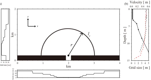
Figure 2. Plan view of the MITgcm (a). Black rectangles extending along the x-axis between 0 < y < 0.2 km represent the modeled shoreline, which is interrupted by the river mouth at 1.9 < x < 2.1 km. The semicircle and arrows extending from the river mouth (dot) are used for depicting Figures 5, 6, and 13; see text for details. The lower and left-hand panels represent the grid sizes in the x and y directions, respectively. Panel (b) shows the layer thickness in the vertical direction (solid curve) and the vertical profile of tidal currents at x = 2 km, y = 1 km, and at 31 hours from the beginning of the computation; black (red) broken curve for case 3 (4) in Table 1.
Figure 3. Plan and vertical views obtained by the field survey. An aerial photograph taken from the balloon towed by a research boat (arrow) is shown in (a). The
photograph was processed by projective transformation and placed in Cartesian coordinates, for which the horizontal and vertical scales are shown in the panel. Red dots indicate the CTD stations in Figure 1. Panel (b) shows the vertical section of salinity observed along the CTD stations (triangles on the abscissa) in Figure 1. Contour interval is 0.2. Isohalines <31.0 are omitted because of overcrowding. Bold white contours are used for isohaline 33.0 to emphasize the bottom of the river plume.
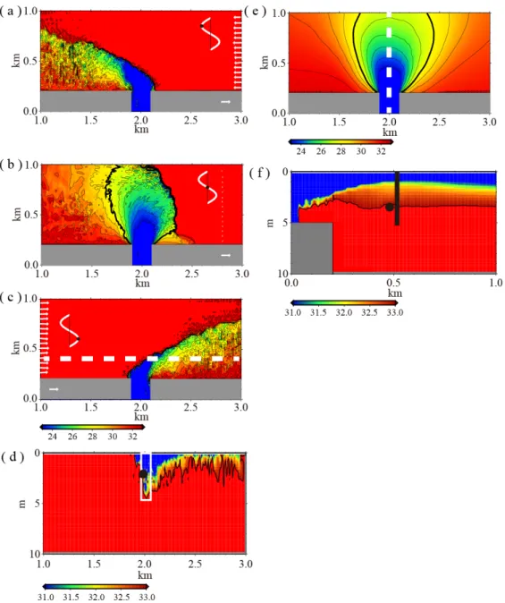
Figure 4. Salinity distribution reproduced in the MITgcm. Plan views of sea surface salinity reproduced in the model with tidal currents at (a) 25, (b) 28, and (c) 31 hours from the beginning of the computation are shown in the left-hand panels. Note that the area with y < 1 km is shown in the plan views. Contour interval is 1, but isohalines
<23.0 are omitted because of overcrowding. White arrows along the lateral boundaries
(stippled area) is depicted to indicate the velocity reference of 1 m s–1. White curves and black dots indicate the respective tidal phase. Panel (d) shows the vertical view at 31 hours along the broken line in (c). The white box and solid circle in (d) are used in depicting Figure 10 and 11, respectively. Isohaline 33.0 is added to emphasize the bottom of the river plume. The sea surface salinity map (e) and vertical view (f) along the broken line in (e) are the same as (b) and (d), respectively, but for the model without tidal currents (case 2 in Table 1). The solid circle and bold line in (f) are used for
depicting Figures 11 and 12, respectively.
Figure 5. Dependency of freshwater abundance (defined as Eq. (1)) versus the distance from the river mouth. The abundance is computed as the ratio of freshwater volume to that of the water column at the same position. The black solid, broken, dotted and red curves in panel (a) indicate the dependency computed in the model with tidal currents (case 1 in Table 1), with halved tidal currents (case 7), with slope (case 8) and without tidal currents (case 2), respectively. Panel (b) shows the same as panel (a), but with the doubled river discharge (case 5 and 6).
Figure 6. Same as Figure 5 but for momentum balance (a, b, c, and d) and the
contribution to the advection term (see text for details) (e). In panel (a), the black (red) curve indicates the magnitude of the advection (pressure gradient) term. The other terms are not shown because they were negligibly small. The panels (b), (c), and (d) are the same as (a), but for x component, y component, and different cases, respectively. In panel (d), the black (red) solid, broken, and dotted curves represent the magnitude of the advection (pressure gradient) term with halved tidal currents (case 7), slope (case 8), and doubled river discharge (case 5), respectively. The panel (e) represents the
magnitude of the horizontal (vertical) component of the advection term by black broken (dotted) curves. The red broken (dotted) curve indicates the magnitude of the horizontal (vertical) component of the advection term associated only with the detided
disturbances. The black solid curve is the same as that in the panel (a).
Figure 7. Rayleigh criterion for inertial instability, Richardson number for K-H instability, and detided disturbances squared in the modeled plume. The grid cells that meet the Rayleigh criterion (Eq. (7); red dots) in the model with tidal currents are shown by red dots at (a) 28.66, (b) 29.16, and (c) 29.66 hours together with the sea surface salinity (contours) at the same time. Also shown by blue dots in the same panels are areas where the Richardson number meets the criterion of Eq. (8) at the bottom of the river plume. Contour interval is 1 and isohalines between 28.0 and 33.0 only are shown in the panels to emphasize the estuarine front. Panels (d)–(f) are the same as (a)–
(c), respectively, but for detided disturbances squared (colors) instead of the Rayleigh criterion. The box in (f) is used for depicting Figure 9. Panel (g) is the same as (d) but for the model without tidal currents (case 2).
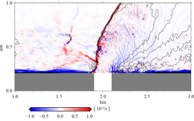
Figure 8. Same as Figure 7b and e but for relative vorticity (colors).
Figure 9. Horizontal distribution of the magnitude of the detided disturbances squared (colors) and sea surface salinity (contours) at (a) 29.66, (b) 29.70, and (c) 29.73 hours within the box in Figure 7f. Contour interval is 1 and isohalines between 23.0 and 33.0 only are shown. The arrow indicates the eddy growing along the estuarine front. The bold curve is used for isohaline 24.0 to show the perimeter of the eddy described in the text.
Figure 10. K-H instability revealed within the white box in Figure 4d. The vertical distribution of salinity in the model with tidal currents (case 1) is shown in (a)–(g) from 30.55 hours with time interval of 10 seconds. The base of the river plume is emphasized by isohaline 33.0 (bold curves). Areas where the Richardson number meets the criterion of the K-H instability (i.e., Ri < 1/4) at the bottom of the river plume are surrounded by white boxes. The dots in Figure 10f are same in Figure 2b from 1.5 to 3.3 m. The bold line in (a) is used for depicting Figure 12. Time series of u'w' at the solid circle in Figure 4d and v'w' in Figure 4f are shown in (h) and (i), respectively. Red curves in (h) indicate the time when the Richardson number was < 1/4.
Figure 11. Time series of the vertical current shear (black curve; the left ordinate) and the Richardson number (red curve; the right ordinate) with (case 1; a) and without (case 2; b) tidal currents at the solid circles in Figure 4d and f. The lines in panel (a) indicates Ri = 0 and 1/4.
Figure 12. Vertical profiles of buoyancy frequency (blue line; the upper abscissa), salinity (black line; the middle abscissa), and vertical shear of horizontal velocity (red line; the lower abscissa) in the model with (a) and without (b) tidal currents at 30.55 hours. Panels (a) and (b) are depicted along the bold lines in Figure 10a and Figure 4f (although Figure 4f is depicted at 28 hours), respectively. The layer where the
Richardson number was <1/4 is stippled.
Figure 13. Same as Figure 5 but for sea surface salinity gradient with (case 1; bold curve) and without (case 2; broken curve) tidal currents.
Figure A. Model domain of the FVCOM for computing tidal currents. The four major tides were given along the open boundary (broken lines) of the domain. The Sea of Japan was not included in the model.
List of Table
Table 1. Computational conditions
1. Introduction
Riverine freshwater containing terrigenous nutrients, sediments, and pollutants can form river plumes that affect coastal ecosystems as well as the ocean circulation.
Consequently, the behavior of river plumes is an important topic in coastal oceanography. It is well known that discharged freshwater in the Northern Hemisphere turns to the right from the viewpoint of an observer at a river mouth looking seaward, and that it forms a coastal boundary current flowing in the sense of a Kelvin wave (e.g., Beardsley & Hart, 1978; Minato, 1983; Chao & Boicourt, 1986; Fong et al., 1997).
Such coastal boundary currents feed nutrients, sediments, and pollutants as well as freshwater to the far field from the river mouth.
Because of the unsteadiness and nonlinearity of river plumes, difficultly arises in terms of ocean dynamics. This is especially the case in the transient region between the river mouth and the coastal boundary current, which is often called a bulge (an anticyclonic eddy) (e.g., Yankovsky & Chapman, 1997; Hickey et al., 1998; Garvine, 2001; Fong & Geyer, 2002; Isobe, 2005), recirculating plume (e.g., Horner-Devine et al., 2009), or near-field plume (e.g. McCabe et al., 2008; Hetland & MacDonald, 2008;
Chen et al., 2009). The introduction by Garvine (2001) remains instructive in the recognition of the “upshelf intrusion” and “forever-growing” bulges; however, problems regarding bulge behavior revealed in numerical models and by laboratory experiments remain unresolved. Based on numerical (Fong & Geyer, 2002; Isobe, 2005;
Horner-Devine, 2009) and laboratory (Horner-Devine et al., 2006) experiments, it has
been established that more than half the riverine freshwater input is trapped inside this transient region. Thus, bulge dynamics govern its growth, the mixing between freshwater and ambient saline water, and the transport of terrigenous materials into coastal waters.
Recent attention has focused on the fluctuation of river-plume bulges due to periodic tidal currents near river mouths (e.g., MacDonald & Geyer, 2004; Orton & Jay, 2005; Halverson & Pawlowicz, 2008; Horner-Devine et al., 2009; McCabe et al., 2009;
Nash et al., 2009; Kilcher & Nash, 2010; Cole & Hetland, 2016). Hereinafter, the term
“bulge” is replaced with “near-field plume”, because bulges, as considered in the recent studies, are recognized as longer rotational retentive structures whose timescale is typically longer than tides (Horner-Devine et al., 2015). As described by Horner-Devine et al. (2009), this “tidal plume” (tidally pulsed near-field plume) could be considered as a subdomain within a river-plume bulge, in which the vertical shear of the horizontal currents (hence, Kelvin–Helmholtz (K-H) billows) generated at the bottom of the river plume enhances the mixing of riverine freshwater with ambient saline water (MacDonald & Geyer, 2004; Orton & Jay, 2005; McCabe et al., 2009; Kilcher & Nash, 2010). Riverine freshwater always spreads to the ocean via a tidal plume formed at the river mouth. Therefore, the mixture within this narrow region (<20 km, even for the Columbia River tidal plume; Kilcher and Nash (2010)) is of particular importance in determining the water properties (i.e., salinity and momentum) in coastal waters.
Despite the finding of fine-scale structures such as K-H instability in tidal plumes,
it remains difficult to state definitively the extent to which these fine-scale structures alter river-plume behavior in coastal waters. This is partly because most previous studies based on numerical modeling approaches have investigated the physical processes under the hydrostatic assumption; see recent studies using numerical models such as the Regional Ocean Modeling System (Cole & Hetland, 2016) and Hybrid Coordinate Ocean Model (Androulidakis et al., 2015). Nonetheless, a few studies have employed nonhydrostatic models to reproduce the generation of internal waves induced by a river plume (Stashchuk & Vlasenko, 2009) and to identify the forcing mechanism of a small river plume (Masunaga et al., 2016). Using nonhydrostatic models, these studies investigated dynamical processes with horizontal scales of around several hundred meters. However, it is also anticipated that nonhydrostatic models could reproduce tidal-plume behavior on horizontal scales of several tens of meters or less.
For instance, if K-H billows generated actually at the bottom of a river plume (MacDonald & Geyer, 2004; Orton & Jay, 2005; McCabe et al., 2009; Kilcher & Nash, 2010) were reproduced explicitly in a model, then friction and enhanced mixing between the plume and the seawater beneath might alter plume behavior.
The objective of the present study was to elucidate how the behavior of a near-field plume might be controlled by the fine-scale structures generated within it. In particular, special attention was focused on the fluctuation of near-field plumes due to tidal currents (i.e., a tidal plume), where fine-scale dynamical structures caused by intense spatiotemporal variability are likely to occur, as suggested by the aforementioned
tidal-plume studies. The present study employed a nonhydrostatic numerical model to reproduce the fine-scale structures down to the order of a few tens of meters, i.e., one order of magnitude smaller than previous numerical studies on river-plume dynamics.
The remainder of the paper is organized as follows. In section 2, the setups of the field observations and numerical modeling are described. The results of the observations and numerical model experiments are presented in section 3. In section 4, the tidally induced instabilities critical in controlling river-plume behavior are investigated, and section 5 summarizes the present study.
2. Material and methods 2.1 Observations
For comparison with the modeled river plume in the present study, two sets of field observations were conducted on a river plume that developed around the Hiji River mouth in the Seto Inland Sea (Japan) on July 1, 2013 (Figure 1). One involved conductivity–temperature–depth (CTD) casts to determine the vertical structure of the river plume in terms of salinity. The other involved low-altitude remote sensing (referred to as “balloon photography”; e.g., see Kako et al. (2012) for the detailed procedure) to provide a plan view of the river plume spreading across the sea surface.
These observations were conducted during daytime from 09:00 to 16:00 Japan Standard Time (JST; UTC + 9). The river discharge averaged over three days before the day of observation was about 49 m3 s–1 (Ministry of Land, Infrastructure, Transport and Tourism; http://163.49.30.82). An advantage of choosing a river with relatively small
freshwater discharge is that the river plume extends within a spatial scale of O(1) km;
thus, a high-resolution nonhydrostatic model can simulate the entire plume without the need for huge computational resources. It was found that northeastward (alongshore) tidal currents with speeds of 0.4–1.0 knots (approximately 0.2–0.5 m s–1) were dominant over the course of these observations (not shown), according to the archived tidal-current data provided on the website of the Japan Coast Guard (http://www1.kaiho.mlit.go.jp/JODC/marine/umi/tide_str_pred.html).
First, CTD casts were deployed 10 times along a survey line, which was set approximately perpendicular to an estuarine front visualized by accumulated foam and debris (Figure 1). In addition, the survey line was determined such that the estuarine front was located at the midpoint of the line. The CTD stations were positioned at approximately 200-m intervals (Figure 1). All CTD casts were completed within 30 minutes from 10:30 JST; thus, the vertical section of the river plume depicted by the CTD surveys can be regarded as a snapshot, despite the temporal variation owing mainly to the semidiurnal tidal currents prevailing over the study area.
Immediately after the CTD casts had been performed, photographs of the estuarine front were taken from a balloon equipped with a digital camera to obtain a fine-resolution plan view of the estuarine front; a pixel on each photograph corresponded to an area of 100 cm2 (see Kako et al. (2012) who used the same method).
Before taking the photographs, we deployed 23 rectangular styrene foam panels each equipped with a single GPS receiver (referred to as “GPS floats”) around the estuarine
front. The positional data recorded by each GPS float were used for the projective transformation (i.e., georeferencing) (Magome et al., 2007; Kako et al., 2012) by which the photographs were converted onto a Cartesian coordinate to evaluate the accurate shape of the estuarine front. If this step was skipped, the shape of the estuarine front in the photographs taken at an oblique angle from the balloon would have been distorted.
The helium-filled balloon was towed by a research vessel moving around the estuarine front, and photographs were taken of both the front and the GPS floats. The wind speed averaged over the observational period was about 2 m s–1 (provided by the Japan Meteorological Agency website; http://www.data.jma.go.jp/obd/stats/etrn/index.php);
thus, the balloon remained stable at a height of 150 m throughout the course of the observations.
2.2 Model setup
The numerical model used to reproduce the river plume fluctuations due to the tidal currents was the Massachusetts Institute of Technology General Circulation Model (MITgcm; Marshall et al., 1997) under the nonhydrostatic assumption. For simplicity, the model domain was a rectangular basin with a 4-km length in the alongshore (x) direction, 2-km length in the cross-shore (y) direction, and 15-m depth to a flat bottom, i.e., nearly the same depth as the observation area (Figure 2). As shown later in Figures 3b and 4d, the river plume in the present study had a layer thickness of <5 m. Therefore, even in the relatively shallow water, the plume could be regarded as a surface-advected
plume (Yankovsky & Chapman, 1997). A nonslip sidewall representing the shoreline was placed along y = 0.2 km, and three open boundaries were set at the remaining ends (i.e., x = 0 and 4 km; y = 2 km) of the model domain. At the midpoint (x = 2 km) of the shoreline, the model domain had a single river mouth, the width and depth of which were 200 and 5 m, respectively. These lengths represent those of the Hiji River mouth.
To reproduce the nonhydrostatic processes, the aspect ratio of the modeled grid cells was set to one fifth near the river month; the horizontal grid spacing changed from 1.5 m near the river mouth to 30 m near the model boundary; and the vertical grid spacing for the 15 layers changed from 0.3 m at the surface to 5 m at the bottom (Figure 2). As shown later in Figure 4, the area with the finest grid spacing was positioned close to the river mouth in order to cover the modeled river plume. Likewise, the vertical resolution becomes dense in the uppermost layer to reproduce the river plume spreading around the sea surface. In the numerical experiments, the Smagorinsky scheme was used for horizontal viscosity, adopting a constant coefficient of 0.3. Horizontal diffusivity was also set to a constant value: Kh = 4 × 10⁻³ m2 s–1 (~0.01 × 5004/3 cm2 s–1). Similarly, constant values were set for both vertical viscosity and diffusivity: Av = Kv = 10–4 m2 s–1. The Coriolis parameter and drag coefficient at the ocean floor were set to 8.05 × 10⁻⁵ s–1 and 2.5 × 10⁻⁴, respectively.
Motion in the model was forced by both buoyancy flux from the river mouth and tides given at the open boundaries. Based on the average value recorded for the Hiji River, the river discharge was set to 49 m3 s–1. The tidal currents that actually occurred
during the observation period in the study area were imposed at both left and right ends of the domain (x = 0 and 4 km) as the sum of the four major tidal constituents, the harmonic constants of which were computed separately using the Finite Volume Coastal Ocean Model (Chen et al., 2003; see the Appendix for the tidal current computation).
The maximum value of the tidal-current speed over the model domain was 0.62 m s–1. The radiation condition (Niwa & Hibiya, 2001, 2004; Carter et al., 2008) for long gravity waves was applied at the offshore open boundary (y = 2 km). To absorb less saline water at the left (x = 0 km) and right (x = 4 km) boundaries, salinity was restored to the ambient value (33.5) on a timescale of 72 hours (i.e., a sponge-layer condition).
The sponge layers at both side boundaries were required because less saline water potentially reached both boundaries owing to the tidal excursion as well as the coastal boundary current on the rotating frame. Salinity was fixed to the ambient value at the offshore boundary (y = 2 km). The model domain had no heat or freshwater fluxes through either the sea surface or the ocean floor.
The model experiments were conducted in accordance with the procedure described below. The computation started at rest with initial temperature and salinity of 25 °C and 33.5, respectively. The temperature was kept constant throughout the course of the computation; thus, the seawater density within the model domain depended only on salinity in the present application. The river discharge of 49 m3 s–1 was maintained continuously from the onset of the computation. This model experiment continued until the end of day 2, because the tidally induced fluctuation of the river plume was found
stable even after day 1, and because the relatively short period was desired owing to the limited computational resource. The above model setup is referred to as the case 1 (Table 1). To examine the dynamical processes relating to the combination of a river plume and tidal currents, we conducted an extra “detided” experiment, where all conditions and computational procedures were the same as the case 1, except for the absence of tidal currents at the open boundaries (x = 0 and 4 km; case 2 in Table 1).
Likewise, we separately computed the tidal currents in the absence of the river plume using a model (case 3) and dividing the entire water column into 15 layers with the same thickness (i.e., 1-m thickness per each; case 4). These extra experiments were conducted to investigate to what extent tidal currents in the uppermost layer were distorted owing to the relatively coarse resolution in the bottom boundary layer (Figure 2b). In addition, to investigate the dependence of boundary conditions including the bottom topography, four additional experiments were conducted. The doubled (98.0 m3 s–1) river discharge was given to the models with and without tidal currents (cases 5 and 6), while the halved tidal-current amplitudes were given to the case 7. To investigate the influence of the bottom slope in the actual situation (Figure 1), the same boundary conditions were given to the case 8 except for the depth varying linearly from 5 m at y = 0.2 km to 15 m at y = 2 km.
3. Results
3.1 Observed river plume at the Hiji River mouth
A single estuarine front defined by accumulated foam and debris is clearly visible
between Stas. 6 and 7 in the balloon photograph (Figure 3a). The appearance of the debris–foam line with width of <10 m suggests the occurrence of intense surface convergence (downwelling) along the estuarine front, as observed by O’Donnell et al.
(1998) and by Orton and Jay (2005). Also, of particular interest is the appearance of meanders (eddies) with wavelength of several tens of meters. As mentioned above, northeastward tidal currents prevailed during the balloon photography. It is therefore reasonable to find the estuarine front on the downstream side at the distance of approximately 1000 m from the Hiji River mouth; see the locations of the river mouth and Stas. 6 and 7 in Figure 1. A tidal plume could become broken when carried a long distance by ambient tidal currents. However, in this case, the distance of 1000 m from the river mouth (Figure 1) is much shorter than the tidal excursion due to the prevailing semidiurnal tides (2.8–6.9 km for amplitudes of 0.2–0.5 m s–1); thus, it was unlikely for the breaking of tidal plume to proceed sufficiently.
The vertical section of salinity shows a notable horizontal gradient between Stas. 6 and 7 (Figure 3b), coincident with the visually located position of the estuarine front.
Overall, it was found that the river plume formed in the thin uppermost layer with a thickness of a few meters (<5 m), because the discharge of the Hiji River was relatively low (49 m3 s–1).
It is worthwhile noting that the bottom of this thin plume is not “flat,” but is instead accompanied by disturbances; see isohaline undulations with horizontal length of O(100) m. These subsurface disturbances might be derived from fine-scale dynamical
structures, such as the K-H instability mentioned in previous observational studies (MacDonald & Geyer, 2004; Orton & Jay, 2005; McCabe et al., 2009; Kilcher & Nash, 2010), although the present survey with station intervals of approximately 200 m was too coarse to resolve such fine structures. In addition to the highly disturbed base of the river plume, it is also interesting that isolated patchiness of less-saline water existed at the surface between Stas. 3 and 4. This was not accompanied by a debris–foam line (not shown in figures). Thus, it is suggested that this patchiness developed over a period too short for the accumulation of foam and debris to occur, although this paper will not delve into the processes of how this patchiness generated because of the limitation of the snapshot survey.
3.2 River plumes reproduced in nonhydrostatic models with and without tidal currents
It was found that the modeled river plume oscillated along the shoreline in accordance with the periodicity of the tidal currents (Figure 4a–c; case 1). It was confirmed that the vertical profile of tidal currents above 5-m depth was nearly identical irrespective of the layer resolution (Figure 2b; cases 3 and 4), and thus, the oscillation of the river plume cloud be reproduced realistically as in the actual tidal regimes. As mentioned in the Appendix, semidiurnal tides (especially the M2 tide) prevail over the model domain. Therefore, the modeled plume oscillated symmetrically in the alongshore direction during the first half of day 2; the plume exhibited a similar pattern during the second half (not shown). The thickness (vertical) of the modeled river plume
(Figure 4d) was the same as actually observed at the Hiji River mouth (Figure 3b); see blue areas (<31.5) in both panels. It should be noted that the river plume without tidal currents primarily, but not explicitly, spread offshoreward in a symmetric fashion about the river axis (Figure 4e; case 2). Although the river plumes reproduced in previous numerical studies on rotating frames always formed a combination of a coastal boundary current and a bulge (e.g., Fong & Geyer, 2002; Isobe, 2005), these phenomena were not revealed in the present application. It is therefore suggested that the river plume in the present study was subject to a nonrotating regime because of relatively short computational time (<2 days) in addition to a large Rossby number (>5), which was computed using the diameter of the plume (~1 km), current speed averaged within the plume (1 km × 1 km area off the river mouth; from 24 hours to 36 hours), and the Coriolis parameter (8.05 × 10⁻⁵ s–1).
In addition to the tidally induced fluctuation of the river plume, a remarkable difference observed between the experiments with and without tidal currents is the occurrence of fine-scale eddies (disturbances) with spatial scales of several tens of meters, which were resolved well by the present model with its 1.5-m horizontal grid spacing. The horizontal distribution of surface salinity shows that the fine-scale eddies are generated over the tidally fluctuating plume (Figure 4a–c; hereafter, referred to as the “tidal plume” in line with Horner-Devine et al., 2009). However, the isohalines of the modeled plume without tidal currents (Figure 4e) seem smoother than those of the modeled tidal plume (see Figure 4b at slack tide). The vertical section of salinity also
shows wavy fluctuations with spatial scales of several tens of meters around the bottom of the tidal plume (Figure 4d). Note, the present model with horizontal (vertical) grid spacing of 1.5 (0.3) m is well capable of resolving these wavy fluctuations around the tidal plume. Conversely, the bottom of the plume without tidal currents (Figure 4f) remains flat in comparison with the tidal plume; note that the location of the cross section is different from Figure 4d because of the location of the river plume. It is considered that the fine-scale disturbances in both horizontal and vertical views are certainly caused by a combination of the river plume and tidal currents, because the two experiments (cases 1 and 2 in Table 1) were conducted under identical computational conditions except for the tidal currents given at the model boundaries. The occurrence of these disturbance is the essence of this paper using a very fine resolution, and will be discussed in the subsections 4.2 and 4.3. It should be noted that, as in the model experiment, fine-scale disturbances were observed in the actual situation (hence, with tidal currents) in both plan (Figure 3a) and vertical (Figure 3b) views.
In addition to the generation of the fine-scale disturbances, a remarkable difference between the numerical experiments with and without tidal currents is the offshoreward extension of the less-saline river water. Comparison between the sea surface salinity at slack tide (Figure 4b) and without tidal currents (Figure 4e) is more telling. It seems likely that isohaline 28.0 (see bold curves) in Figure 4e extends more broadly than in Figure 4b. However, Chen (2014) demonstrated that tidal currents enhance the fresh water transport in the coastal currents because of changeing the pressure field of the
river plume. To examine further the offshoreward extension of freshwater quantitatively, the percentage of detided freshwater volume within a water column, 𝑄(𝑟), averaged along the perimeter with radius r from the river mouth (Figure 2) was calculated as follows:
𝑄(𝑟) = * 1
𝑇ℎ𝑙/0 0 0 𝑆2 − 𝑆 𝑆2
2 45 67 2 8 2
𝑑𝑧 𝑑𝑙 𝑑𝑡=, (1)
where T denotes the period of the prevailing tide (12 hours was used for simplicity in this application), h is the depth of the modeled domain (15 m), lr is the length of the perimeter of the semicircle with radius r (shown in Figure 2). Here, S0 and S represent the ambient (i.e., 33.5) and the computed salinity values, respectively. This computation was conducted using the modeled results of the first half of day 2. Intuitively plausible is that tidally induced fluctuations have a role in the efficient diffusion of freshwater offshoreward into the ambient saline water. However, of particular interest in the present experiments is that the tidal currents had a role in confining the river plume close to the river mouth (black solid curve [case 1] in Figure 5a). Were it not for the tidally induced fluctuations, the modeled river plume would have spread a long distance in the offshoreward direction (red curve [case 2] in Figure 5a). The dependence of the tidal-plume spread on the presence of tides was revealed in the model with the doubled river discharge (Figure 5b; case 5 and 6). It is therefore suggested that the confining around the river mouth occurs for tidal plumes with the river discharge < O(100) m3 s–1. In addition, it is noted that the tidal-plume spread depends on tidal-current amplitudes;
see Figure 5a where the offshoreward spread of the tidal plume changes to be modest in
the model with the halved tides (broken curve in Figure 5a; case 7). Meanwhile, the confining of tidal plume around the river mouth was enhanced in the model with the bottom slope (dotted curve in Figure 5a; case 8). This is consistent with the dependence on tides mentioned above, because the tidal-current amplitude close to the river mouth become larger than that in the case 1 due to the shallow depths.
4. Discussion
4.1 Momentum balance in the river plume
It is worthwhile to calculate the momentum balance in the modeled tidal plume to answer the question why the river plume is confined by the tidal currents to near the river mouth. The tidally averaged momentum balance over the period in the first half of day 2 was averaged spatially along the perimeter in Figure 2. Thus, each term in the momentum balance was calculated as a function of the radial distance r from the river mouth in the same manner as shown in Figure 5 (Figure 6a). The magnitudes of the terms including the current velocities (𝑢, 𝑣, 𝑎𝑛𝑑 𝑤) were decomposed into terms associated with tidal currents only (𝑢DEFG, 𝑣DEFG, 𝑎𝑛𝑑 𝑤DEFG), tidally averaged currents (i.e., subtidal currents; 𝑢H, 𝑣̅, 𝑎𝑛𝑑 𝑤J), and the anomalies from these two magnitudes (the anomalous currents are hereafter referred to as detided disturbances; 𝑢K, 𝑣K, and 𝑤K), to examine the contributions of each current velocity to each term. These currents components are shown as follow:
𝑢 = 𝑢H + 𝑢DEFG + 𝑢K 𝑣 = 𝑣̅ + 𝑣DEFG + 𝑣K 𝑤 = 𝑤J + 𝑤 + 𝑤K
. (2)
The terms associated with tidal currents only were computed separately using the same numerical model with tidal currents but without river discharge. The removal of the terms associated with tidal and subtidal currents from those computed originally by the modeled currents provides the contribution of the detided disturbances to each term.
The momentum balance was computed only in the uppermost layer for ease of the analyses, because the river plume was confined within the thin upper layer (Figure 4d):
we confirmed that the momentum balance at 3-m depth, mid-depth of the plume, was nearly the same as that in the uppermost layer (not shown).
Prevailing in the momentum equation are the advection (A) and pressure gradient (Ph) terms (Figure 6a) around the river mouth (r <500 m), the magnitudes of which can be evaluated as:
𝐴(𝑟) = 1
𝑇𝑙/0 0 P(𝒖 ∙ 𝛁𝑢)T+ (𝒖 ∙ 𝛁𝑣)T
67
2 8
2
d𝑙 d𝑡, (3)
𝑃5(𝑟) = −1
𝑇𝑙/0 0 𝜌24Y|𝛁5𝑃|
67
2 8
2
𝑑𝑙 𝑑𝑡, (4)
where 𝛁 and 𝛁5 denote ∂/∂x i + ∂/∂y j + ∂/∂z k and ∂/∂x i + ∂/∂y j, respectively, i and j are the horizontal unit vectors, and k is the vertical unit vector; otherwise, the notation is standard. The subtidal currents, tidal currents, and detided disturbances are all included in the above estimate. The local acceleration, Coriolis, and viscous terms are not revealed in Figure 6a because they were all negligibly small in comparison with the above two terms. The minor contribution of the Coriolis term is consistent with the fact
that the river plume spreads mostly in the offshoreward direction in the absence of the modeled tidal currents (Figure 4e). Although the equilibrium state between the advection and pressure gradient terms was also revealed in both x and y directions (Figure 6b and c), we hereinafter investigate the sum of these two components (i.e., Eqs.
(3) and (4)) for simplicity. In addition, the equilibrium state was revealed in three additional experiments with tidal currents (Figure 6d; cases 5, 7, and 8); thus, the discussion hereinafter would commonly be accomplished irrespective of tidal-current amplitude, river discharge (<O(100) m3 s–1), and bottom topography.
It was found that the detided disturbances mostly account for the advection terms in both horizontal and vertical directions. First, the advection term, Eq. (3), was decomposed further into the horizontal (Ah) and vertical (Av) components as follows:
𝐴5(𝑟) = 1
𝑇𝑙/0 0 P(𝒖𝒉∙ 𝛁𝒉𝑢)T+ (𝒖𝒉∙ 𝛁𝒉𝑣)T
67
2 8
2
d𝑙 d𝑡, (5)
𝐴^(𝑟) = 1
𝑇𝑙/0 0 _𝑤𝜕𝒖𝒉
𝜕𝑧 _
67
2 8
2
d𝑙 d𝑡, (6)
where 𝒖5 and w are the horizontal and vertical current components, respectively (Figure 6e). The horizontal and vertical advection terms both dominate near the river mouth, although the horizontal component prevails over the vertical one (Figure 6e). It is interesting that the detided disturbances dominate over the other contribution to the advection term, especially near the river mouth in both horizontal and vertical directions (red curves in Figure 6e). Thus, it is found that the contribution owing to subtidal
currents, tidal currents and a combination of tidal/subtidal currents and detided disturbances such as 𝑢DEFG𝑑𝑢K𝑑𝑥 were all relatively small compared to the contribution owing to the detided disturbances. It should be noted that a combination of the river plume and tidal currents generates these disturbances, because the magnitudes of these anomalous advection terms from the 12-hour average were negligibly small in the model without the tidal currents (not shown). The predominance of the advection associated with the detided disturbances suggests that an equilibrium state was accomplished between the horizontal pressure gradient (Eq. (4)) and eddy viscosity (momentum exchange) terms, such as 𝑢′𝑢′ (= 𝜈5 𝜕𝑢/𝜕𝑥) and 𝑢′𝑤′ (= 𝜈^ 𝜕𝑢/𝜕𝑧), in both horizontal and vertical directions in the river plume, where the overbar denotes the tidal average, and 𝜈5 (𝜈^) is the horizontal (vertical) viscosity coefficient.
4.2 Horizontal momentum exchange due to inertial instability
A dynamical process causing the horizontal momentum exchange results from the occurrence of inertial instability, as shown below. We hereafter demonstrate the “detided disturbances squared” such as 𝑢K𝑢K, 𝑣K𝑣K, and 𝑢K𝑣K to investigate the momentum flux across the estuarine front. The divergence of their temporal average yields the Reynolds stresses. It is interesting that the magnitude of the detided disturbances squared P(𝑢K𝑢K)T+ (𝑢K𝑣K)T + (𝑣K𝑣K)T becomes large in phase with the occurrence of inertia instability explored by the Rayleigh criterion on a nonrotating frame (Figure 7):
𝑟𝜕𝑣f
𝜕𝑟 + 𝑣f < 0, (7)
where r is the curvature radius of a water parcel, computed as 𝑟 = (𝑢T+ 𝑣T)j/T∕ (𝑢𝜕𝑣/𝜕𝑡 – 𝑣𝜕𝑢/𝜕𝑡), and 𝜕𝑣f/𝜕𝑟 and 𝑣f are approximated to 𝜕𝑣/𝜕𝑥 – 𝜕𝑢/𝜕𝑦 and
√𝑢T+ 𝑣T, respectively. At slack tide, when the river plume spreads in the offshoreward direction, the estuarine front on the left-hand side of the plume meets the criterion of Eq.
(7) (Figure 7a). Thereafter, as the river plume moves to the right, because of the tidal currents flowing from left to right, the areas satisfying Eq. (7) remain aligned along the estuarine front (see red dots in Figure 7b and c). The positive (anticlockwise) relative vorticity along the estuarine front indicates the occurrence of cyclonic eddies (Figure 8;
at the same time as Figure 7b). Thus, the intensive current shear generated by a combination of the river plume and the ambient tidal currents triggers the inertial instability. It should be noted that the large magnitude of the detided disturbances squared appears around those areas where the inertial instability is likely to occur (Figure 7d–f). The detided disturbances are developed at 29.2 hours when the entire estuarine front meets the criterion of Eq. (7) (Figure 7e). It is also interesting that the areas with large magnitudes extend downstream of the tidal currents from the estuarine front (namely, inside the plume; Figure 7d–f). This provides a scenario in which the detided disturbances (hence, the momentum outside the plume) penetrate into the river plume, such that the inertial instability exerts friction with the ambient saline water.
This suppresses the extension of the tidal plume via momentum exchange.
The appearance (disappearance) of the large magnitudes of the detided disturbances squared in the model with (without) tidal currents in Figure 7d–f (Figure 7g) is
consistent with the appearance (disappearance) of fine-scale eddies with spatial scale of several tens of meters in Figure 4a–c (Figure 4e). In fact, the momentum exchange due to the detided disturbances is visualized well by the growth of these fine-scale eddies along the estuarine front. For example, Figure 9, enlarged from the box shown in Figure 7f, provides subsequent snapshots with intervals of 0.03 hours. An eddy (arrow in Figure 9a) grows rapidly as it moves toward the upper right (i.e., the “downstream”
direction of the combined tidal currents and freshwater spreading from the river mouth;
Figure 9b and c). The timescale taken for the eddy to grow is <2 minutes, i.e., from Figure 9a to 9b; thereafter, the eddy appears mature (Figure 9c). This evolution process is apparently shorter than the tidal period (~12 hours in the present case); thus, the detided disturbances (𝑢K, 𝑣K) revealed in the model with tidal currents (Figure 6b) are likely associated with eddies, such as those shown in Figure 9. In fact, the magnitude of the detided disturbances squared, (P(𝑢′𝑢′)T+ (𝑢′𝑣′)T+ (𝑣′𝑣′)T), varies in space on a scale of several tens of meters along the estuarine front, consistent with the spatial scale of the eddies (color tone in Figure 9). It is therefore considered that the growth of these eddies results in the horizontal exchange of momentum (also, freshwater) between the river plume and the ambient saline water. The location of the frontal eddies does not always correspond to large values of detided disturbance squared. This is probably because the momentum exchanged by eddies further penetrates into the plume interior.
Of particular interest is that the fluctuation visualized from the balloon photograph also had a spatial scale of several tens of meters around the estuarine front of the Hiji River
(Figure 3a).
4.3 Vertical momentum exchange due to Kelvin–Helmholtz instability
Previous studies have suggested that K-H instability occurs at the bottom of the river plume near the river mouth (e.g., MacDonald & Geyer, 2004; Orton & Jay, 2005;
McCabe et al., 2009; Kilcher & Nash, 2010). Thereby, it is reasonable to consider that the large magnitudes of the vertical advection term near the river mouth (Figure 6e) are associated with the generation of K-H instability. In fact, the bottom of the river plume undulates intensely on a scale of several tens of meters in the numerical experiment with tidal currents (Figure 4d). It should be noted that the field observations also showed isohaline undulations, although the CTD casts with relatively coarse intervals (~200 m) were insufficient to resolve their spatial scale (Figure 3b).
The undulation developed at the bottom of the river plume is caused by the development of K-H instability, which can be explored by the Richardson number (Ri):
𝑅𝑖 = 𝑁T
(𝑑𝑢/𝑑𝑧)T+ (𝑑𝑣/𝑑𝑧)T < 1
4, (8)
where N2 = –g/ρ∂ρ/∂z is the buoyancy frequency, g is gravitational acceleration, and ρ is density. The box in Figure 4d is enlarged in Figure 10a, and subsequent snapshots with intervals of 10 seconds are presented in Figure 10b–g. White boxes in these panels indicate the grid cells that meet the criterion of Eq. (8). In order to emphasize the K-H instabilities at the bottom of the river plume (defined as isohaline 33.0), white boxes only on this isohaline are indicated. It is found that eddies (arrows A and B in Figure
10a–g) develop in areas where Ri < 1/4. Eddy A in Figure 10a, which is outside the area where Ri < 1/4, did not grow in Figure 10b. Thereafter, it can be seen to rapidly grow and decay in Figure 10c–e as areas where Ri < 1/4 appear and disappear repeatedly.
Similarly, eddy B starts to grow at the time when an area where Ri < 1/4 appears (Figure 10c and d), and it develops immediately within the white box moving to the right (Figure 10d–f). Note that the eddy is sufficiently resolved in the present model with the high vertical resolution; see white dots in Figure 10f.
The time series of the detided disturbance squared provides a more cogent result (Figure 10h and i) than the snapshots of the abovementioned eddies. The disturbances were monitored at the bottom of the river plume, defined by isohaline 33.0 (see solid circles in Figure 4d and f) with (Figure 10h) and without tidal currents (Figure 10i) during half of the prevailing tidal period (27–33 hours). In the presence of tidal currents, almost all of the 𝑢K𝑤K (≫ 𝑣K𝑤K) peaks were revealed when the Richardson number at the same position met the criterion of Eq. (8) (see red dots in Figure 10h). Meanwhile, the disturbances (𝑣K𝑤K (≫ 𝑢K𝑤K)) in the absence of tidal currents were three orders of magnitude smaller than those with tidal currents and the criterion remained unsatisfied throughout the period (Figure 10i).
The occurrence of K-H instability results from the intensification of the vertical shear of horizontal currents around the bottom of the tidal plume. We first demonstrate the time series of the vertical current shear and Richardson number at the closed circles depicted in Figure 4d and 4f. The current shear and Richardson number were computed
using two values in the upper and lower layers neighboring the closed circle vertically.
We averaged the value along the neighboring five grid cells in the y (x) directions (i.e., across the plume) before computing the vertical gradient in Figure 4d (f). In the presence of the tidal currents, the vertical current shear become higher especially after 29 hours (black curve in Figure 11a). At the same time, the Richardson number frequently takes the values between 1/4 and 0 (red curve in Figure 11a). Thus, it is suggested that the K-H instability certainly occurred owing to the enhancement of the vertical current shear, although the convective overturning was likely to follow the K-H instability producing folded eddies (see Figure 10) as suggested by the spiky pattern of Ri curve that occasionally becomes less than 0 (i.e., tutv> 0 in Eq. (8)). In contrast, in the absence of the tidal currents, the Richardson number was always higher than 1/4 because the current shear is one order of magnitude smaller than the tidal plume (Figure 11b).
Moreover, the occurrence of K-H instability is examined by a snapshot of Eq. (8) within river plumes. We show the vertical profiles of salinity along the bold bars in Figure 10a (same location as the solid circle in Figure 4d) and Figure 4f at 30.55 hours.
This time was chosen arbitrarily but it represents a period when both the large disturbance and a value of Ri < 1/4 appeared in the model with tidal currents. It is found that the peaks of the buoyancy frequency (i.e., vertical salinity gradient) and vertical current shear (=xt𝒖tvyx) appear at a depth <1 m, regardless of whether tidal currents
existed (Figure 12a and b). However, of particular interest is the occurrence of the second peaks of the buoyancy frequency and vertical current shear, which occurred only in the model with tidal currents at the bottom of the less-saline river plume at a depth of around 2.5 m (Figure 12a). The layers between the upper and lower peaks are statically unstable because of the saline inversion; thus, both the buoyancy frequency and the current shear decrease drastically within the mid-depth of the tidal plume because of vertical mixing and K-H instability. In the model with tidal currents, the layers where Ri
< 1/4 extend deeper than in the model without tidal currents (see stippled layers in Figure 12a and b). The increase of the vertical shear, the contribution of which prevails over the buoyancy frequency, results in the tidal plume meeting the criterion of Eq. (8) at the bottom of the river plume (Figure 10h). Although a layer that meets the criterion of Eq. (8) exists in the model without tidal currents, because of the upper peak of the current shear, this layer is restricted within the uppermost layer (<1 m). Thus, it might have a small influence on the disturbances at the bottom of the river plume. In fact, the disturbances without tidal currents (𝑣K𝑤K) are much less than with tidal currents, and the criterion (Ri < 1/4) is not satisfied at the bottom of the river plume (Figure 10i).
The enhancement of the vertical current shear results from the combination of the river plume and tidal currents. It is likely that the intense tidal currents carry the river plume downstream from the river mouth (see Figure 4a–c); thus, the horizontal gradient of sea surface salinity (hence, density) increases, as shown in Figure 13 where the sea surface salinity gradients were computed in the same manner as Figure 5. The
horizontal currents were modified by the pressure gradient associated with the tidal fluctuations of the plume, and thus, the momentum balance was likely to be accomplished transiently between the momentum tendency (𝜕𝑢5/𝜕𝑡) and pressure gradient. Therefore, vertical differentiating this momentum balance states that the vertical shear increases temporally in accordance with a relationship on the nonrotating as:
𝜕
𝜕𝑡z𝜕𝒖5
𝜕𝑧 { ∝ 𝜕
𝜕𝒙z𝜕𝑃
𝜕𝑧{ ∝ 𝜕𝜌
𝜕𝒙, (9)
where the hydrostatic component is used for the conversion from the second to the third terms from the left-hand side, and the notation is standard in the conventional manner.
The increase of the current shear between 29 and 30 hours in Figure 11a is consist with the fact that the surface salinity contours become crowded from Figure 4b (28 hours) to c (31 hours).
The horizontal density gradient increased along the river-plume front; thus, the inertial instability, which is generated around the front because of intense current shear, is likely to coexist with the K-H instability. In fact, the areas in which Ri < 1/4 at the bottom of the river plume (blue dots in Figure 7a–c) are spread sporadically in Figure 7a, but become concentrated around the front in Figure 7b. Thereafter, the blue dots are distributed over the entire domain of the modeled plume in Figure 7c. The appearance of Ri < 1/4 around the areas where inertial instability occurred (Figure 7b) implies the frontal meander (hence, local intensification of frontal sharpness) due to inertial instability triggered the K-H instability beneath it. However, an in-depth examination
will be required to elucidate more conclusively the interaction between these two instability processes.
5. Conclusions
The present study elucidated how the fine-scale disturbances generated by tidal currents influence the behavior of a river plume. The role of the disturbances was investigated based on field observations and numerical experiments. First, balloon photography and CTD casts were conducted to determine the plan and vertical views, respectively, of a river plume. The estuarine front visualized from accumulated debris and foam in the aerial photographs was accompanied by a meander with a wavelength of several tens of meters. The vertical view showed that the relatively thin river plume (thickness <5 m) had an undulated bottom because of the development of small eddies, although they were inadequately resolved by the CTD casts with sampling intervals of around 200 m. Second, nonhydrostatic numerical experiments with and without tidal currents were conducted to reproduce the abovementioned fine-scale structures of the river plume and to investigate the dynamical processes via which they are generated by the tidal currents. The river plume without tidal currents expanded offshoreward like a balloon, as seen in previous numerical studies on a rotating frame, while the tidally fluctuating river plume (i.e., the tidal plume) was confined to near the river mouth. The tidal plume was dynamically equilibrated between the pressure gradient term and the advection terms composed mainly of the contributions of the detided disturbances,
which act as friction owing to the momentum exchange between the plume and the ambient saline water. The horizontal and vertical components of the detided disturbances are generated by inertial instability and K-H instability, respectively. It is considered that a combination of the river plume and tidal currents enhances the current shear favorable for these instabilities to occur.
The occurrence of the inertial and K-H instability processes was suggested based on relatively coarse observed snapshots (Figure 3), which were inadequate for validating the spatiotemporal variations revealed in the numerical model (Figures 9 and 10). Therefore, this limitation should be addressed in future studies by conducting intensive field surveys to investigate the inertial and K-H instability processes generated around tidal plumes. A combination of “tow-yo” (e.g., MacDonald et al., 2013) CTD/ADCP casts, and low-altitude remote sensing, such as the balloon photography used this study, could be a powerful tool for evaluating the Rayleigh criterion (Eq. (7)) and Richardson number (Eq. (8)) in an actual situation. However, we will still encounter the difficulty arising from the fact that the spatiotemporal scales of these processes are one order of magnitude smaller than the field observations obtained in the coastal waters. The inertial instability had a spatial (temporal) scale of several ten of meters (a few minutes) (Figure 9), while the K-H instability had nearly the same spatiotemporal scale (Figure 10). We will have to establish a novel observational technology and/or operational procedure beyond current limitations to resolve these coastal processes.
Finally, we have to acknowledge the limitations of the present numerical model
approach. First, the grid spacing might remain insufficient for resolving K-H billows.
Recently, Zhou et al. (2017) reproduced the shear instabilities developed at the bottom of a freshwater plume using an idealized nonhydrostatic numerical model with horizontal and vertical resolutions less than one-third those used in the present study. A folded-wave pattern was observed clearly at the bottom of the plume, as in laboratory experiments (e.g., Yuan & Horner-Devine, 2013). The modeled K-H billows (Figure 10) would become more intense than in the present study if much finer grid spacing were adopted. Thus, vertical friction might be exerted on the tidal plume more effectively than projected. Second, the model setup was based on observations of the Hiji River because of the limitation of available computer resources. Thus, our model results are applicable only to relatively small rivers with discharge of 49.0–98.0 m3 s–1. However, to date, tidal influences on river plumes have been found on a spatio-temporal scale much larger than the present study. For instance, a mechanism controlling the freshwater transport was proposed by Isobe (2005) in terms of inertia instability, and by Chen (2014) in terms of the tidally-modulated pressure field around plumes. Therefore.
future work is intended to clarify the generality of the model for various combinations of tidal currents and larger river discharges.
Appendix: Computation of tidal currents
In the present study, the Finite Volume Community Ocean Model (FVCOM; Chen et al., 2003) was used to compute tidal currents near the Hiji River mouth. The horizontal resolution of the unstructured triangle grid cells changes from 10 km at the model boundaries to 500 m close to the river mouth; see Figure A for the model domain.
The present FVCOM divided the entire water column into 20 σ layers. The 500-m gridded data provided by the Japan Oceanographic Data Center (J-EGG500;
http://www.jodc.go.jp/data_set/jodc/jegg_intro.html) were used for the modeled bathymetry. The four major tidal constituents (M2, S2, K1, and O1) provided by the Ocean Tide Modeling NAO.99Jb (Matsumoto et al., 2000) were specified at the open boundaries; the amplitudes of the semidiurnal (M2 and S2) tides are approximately five times larger than the diurnal (K1 and O1) tides. Using the stable tidal fluctuation, which had been accomplished after 30 days from the beginning of the computation, harmonic constants of each tidal current constituent were calculated in the areas located a distance 2 km (half of the MITgcm’s alongshore length; see Figure 2) from the Hiji River mouth.
The harmonic constants averaged spatially over the cross-shore length of the MITgcm (i.e., 2 km) were given at the open boundaries of the MITgcm to compute the tidal currents. The computation of tidal currents in the MITgcm started simultaneously with the freshwater release from the river mouth.
Acknowledgements
It has been truly fortunate for me to be a student of my respectful advisor, Professor Atsuhiko Isobe. I appreciated his comments to my investigations. The time when I studied physical oceanography with him is the greatest treasure in my life. Also, my special thanks are extended to Associate Professors Shinichiro Kida and Kiyoshi Tanaka for their valuable comments to improve this study.
I have been happy to study with members of the Ocean Dynamics Group in the Center for East Asian Ocean-Atmosphere Research, Assistant Professor Katsuto Uehara, Messrs. Kei Yufu, Hikaru Nakata, Hirofumi Aotani, Shin Ishimoto, Kohei Matsubara, Kenta Araki, Koki Shiroyama, Takahiro Tsutsumi, Yusuke Fujita, Yusei Yamaguchi, Ms.
Michiyo Tanaka, Sayaka Yamaguchi, Kayoko Takashima, Satomi Fujisaki.
I appreciate the captain and crew of the R/V ISANA belonging to the Center for Marine Environmental Studies, Ehime University, for their cooperation with the field observations in the Seto Inland Sea. I also thank Dr. Akira Masuda for fruitful discussions.
Figure 1. Observation area around the Hiji River mouth. The CTD stations (red dots) and 15-m isobath are shown in the right panel.
Figure 2. Plan view of the MITgcm (a). Black rectangles extending along the x-axis between 0 < y < 0.2 km represent the modeled shoreline, which is interrupted by the river mouth at 1.9 < x < 2.1 km. The semicircle and arrows extending from the river mouth (dot) are used for depicting Figures 5, 6, and 13;
see text for details. The lower and left-hand panels represent the grid sizes in the x and y directions, respectively. Panel (b) shows the layer thickness in the vertical direction (solid curve) and the vertical profile of tidal currents at x = 2 km, y = 1 km, and at 31 hours from the beginning of the computation;
black (red) broken curve for case 3 (4) in Table 1.
Figure 3. Plan and vertical views obtained by the field survey. An aerial photograph taken from the balloon towed by a research boat (arrow) is shown in (a). The photograph was processed by projective transformation and placed in Cartesian coordinates, for which the horizontal and vertical scales are shown in the panel. Red dots indicate the CTD stations in Figure 1. Panel (b) shows the vertical section of salinity observed along the CTD stations (triangles on the abscissa) in Figure 1. Contour interval is 0.2.
Isohalines <31.0 are omitted because of overcrowding. Bold white contours are used for isohaline 33.0 to emphasize the bottom of the river plume.
Figure 4. Salinity distribution reproduced in the MITgcm. Plan views of sea surface salinity reproduced in the model with tidal currents at (a) 25, (b) 28, and (c) 31 hours from the beginning of the computation are shown in the left-hand panels. Note that the area with y < 1 km is shown in the plan views. Contour interval is 1, but isohalines <23.0 are omitted because of overcrowding. White arrows along the lateral boundaries represent sea surface current velocities at the same location. The arrow on the shore (stippled area) is depicted to indicate the velocity reference of 1 m s–1. White curves and black dots indicate the respective tidal phase. Panel (d) shows the vertical view at 31 hours along the broken line in (c). The white box and solid circle in (d) are used in depicting Figure 10 and 11, respectively. Isohaline 33.0 is added to emphasize the bottom of the river plume. The sea surface salinity map (e) and vertical view (f) along the broken line in (e) are the same as (b) and (d), respectively, but for the model without tidal currents (case 2 in Table 1). The solid circle and bold line in (f) are used for depicting Figures 11 and 12,
Figure 5. Dependency of freshwater abundance (defined as Eq. (1)) versus the distance from the river mouth. The abundance is computed as the ratio of freshwater volume to that of the water column at the same position. The black solid, broken, dotted and red curves in panel (a) indicate the dependency computed in the model with tidal currents (case 1 in Table 1), with halved tidal currents (case 7), with slope (case 8) and without tidal currents (case 2), respectively. Panel (b) shows the same as panel (a), but with the doubled river discharge (case 5 and 6).