Numerical Study of Tidal Dynamics in the JavaSea Using COHERENS Model

九州大学学術情報リポジトリ

Kyushu University Institutional Repository

Numerical Study of Tidal Dynamics in the Java Sea Using COHERENS Model

ユサフ, ムスタド

https://doi.org/10.15017/1398416

出版情報：九州大学, 2013, 博士（理学）, 課程博士 バージョン：

権利関係：全文ファイル公表済

Numerical Study of

Tidal Dynamics in the Java Sea Using COHERENS Model

MUSTAID YUSUF

July 2013

Numerical Study of

Tidal Dynamics in the Java Sea Using COHERENS Model

A Dissertation

Submitted for the degree of Doctor of Science

by

MUSTAID YUSUF

Kyushu University July 2013

i

Abstract

The Java Sea is located in the western part of Indonesian Waters. It connects to the Indian Ocean through the Sunda Strait. Through the Karimata, Bangka and Gaspar Straits, it connects to the South China Sea and directly connects to the Flores Sea and southern part of the Makassar Strait. Tide plays important roles in shelf seas such as the Java Sea. Several previous studies about the tide and tidal current in the Indonesian Seas by means of numerical modeling have been conducted. However, all the authors have no detail description about the tidal front and tidal energy propagation particular in the Java Sea.

The major purpose of this study is to describe the characteristics of tide and tidal current in the Java Sea with emphasizing on tidal wave and tidal energy propagation as well as tidal front formation. The thesis consists of the following contents:

In the Chapter 1, a general introduction of the present study, and the relation and difference with the previous studies are described.

In the Chapter 2, modeling of tidal dynamics in the Java Sea is explained in detail. Geography and morphology of the Java Sea as well as observation data for

ii

model verification are described. Numerical model that is applied, data input and forcing, and model verification are also described. In the present study, numerical experiments have been performed to study the characteristics of tide and tidal current in the Java Sea using the new version of COHERENS (Coupled Hydrodynamical-Ecological model for Regional and Shelf Seas) V2.0.

The model results are described also in this chapter. We have found that tidal wave and tidal energy fluxes propagate westward in the Java Sea and also clearly show the bifurcation of M2 tidal wave in the Makassar Strait. K1 tidal energy flux is coming from the Pacific Ocean while M2 tidal energy flux is from the Indian Ocean. We show in detail that the tidal waves lose their energy when entering the Java Sea due to the steep bottom topography in the inlet (eastern part of the Java Sea). This part is important because the previous author never showed in such detail.

Tide-induced residual current generated by K1 tide shows a remarkable counterclockwise rotational flow due to geometrical boundary effect and bottom topography despite a clockwise flow by M2 tide in the western part due to the bottom topography and shoaling effect. Tide-induced residual current generated by K1 tide flows westward in the northern part along the coast of Kalimantan and

iii

shifts to south in the western part along the east coast of Sumatera then shifts to east in the western part of the Java Sea along the north coast of Java, then shifts to north just when it reaches the Makassar Strait to complete the rotation.

Tide-induced residual current generated by M2 tide has the similar pattern, but a remarkable clockwise rotational flow appears in the western part. We suppose that the increasing of M2 tidal amplitude due to the shoaling effect and solid boundary generate this pattern.

Tidal front in the Java Sea is also described in this chapter. Comparison between the value of log(H/U³), (where H is the water depth in m and U is the amplitude of tidal current in ms^-1), with the composite image of MODIS-aqua and MODIS-tera of SST gradient distribution for transitional (wet to dry) season in the Java Sea reveals that the tidal front is located at log(H/U³) value of 3.5. That critical value is nearly the same with the values generally found in other areas.

In the Chapter 3, finally the conclusions are followed.

iv

Acknowledgements

I am very pleasure to express my sincere thanks to my supervisor Professor Tetsuo YANAGI for giving an opportunity to study in Kyushu University. I really appreciated and extend profound gratitude for his kind encouragement during my period of study and especially the valuable comments, suggestions and directions to the manuscript.

I also would like to express my sincere thanks to Professor Naoki HIROSE for his kind encouragement, corrections and worthwhile comments to the manuscript, Harumi FUJII-san and Daisuke ISHII-san for their kindness and valuable help during my period of study. My thanks also go to my colleagues Kioshi MISHIRO, Yoshihiko IDE, Dessy Berlianty and Wang Bin for their kindness and helps.

Finally, this work dedicated to my lovely family, my wife Irma Ningsih Aras, my daughter Muallaf Alfiana Ilminadia and my sons Fatih Arif Almaliki and Aflah Mahib Muyassar. My very special thanks to my parents Yusuf Hasan and Habibah.

v

Contents

1 Introduction

2 Modeling of Tidal Dynamics in the Java Sea

2.1 Geography and Morphology of the Java Sea 2.2 Observation Data

2.3 Numerical Model 2.4 Results and discussion

2.4.1 Verification of elevation and current velocity 2.4.2 Tidal type

2.4.3 Tidal wave propagation 2.4.4 Tidal energy propagation 2.4.5 Tide-induced residual current 2.4.6 Tidal fronts

3 Conclusions

References

1 5 5 6 7 11 11 16 21 28 34 39 44 46

vi

List of Figures

Figure1. Indonesia Waters (upper figure) and model domain (lower figure marked by solid line).

Figure 2. Verification of tidal elevation

Figure 3. Verification of tidal current

Figure.4 Tidal amplitude verification (unit in meters)

Figure 5. Distribution of _(M´^(K1+O1)

2+S₂)

Figure 6. Calculated amplitude spectrum distribution of major tidal components

Figure 7. Co-range charts of K1 and M´2 tidal amplitude (unit is meter) Figure 8. Co-tidal charts of K1 and M2 tidal phase (unit is degrees referred

to Indonesian mean time GMT+8 hours)

Figure 9. Co-range chart (upper figure) and co-tidal chart (lower figure) of K1 tide in Indonesian Seas (after Ray, et all., 2005)

Figure 10. Co-range chart (upper figure) and co-tidal chart (lower figure) of M2 tide in Indonesian Seas (after Ray, et all., 2005))

Figure 11. Depth-integrated energy flux vectors for K1 and M´2 tide during one tidal cycle

Figure 12. Vertically integrated energy dissipation of K1 and M´2 tide during one tidal cycle

4

12 14 15

19

20

22 23

24

25

30

33

vii

Figure 13. Depth-mean tide-induced residual current generated by K₁ tide (after 5x5 grids box averaging). Upper figure shows the whole model area, lower figure shows more detail for the Java Sea

Figure.14 Depth-mean tide-induced residual current generated by M´₂ tide (after 5x5 grids box averaging). Upper figure shows the whole model area, lower figure shows more detail for the Java Sea

Figure 15. Co-range chart of K₁ and M´₂ tidal current amplitude

Figure16. Isoline of Log(H/U³). White color denotes the value over than 4.5 Figure.17 Sea Surface Temperature distribution on nighttime of March, composite of MODIS-Aqua 4km (4 micron night) in year 2008, 2011 and MODIS-Tera 4km (4 micron night) in year 2009 images. White color on the sea indicates the clouds omission.

35

36

40 42

43

1

CHAPTER 1 Introduction

The Java Sea is a primary water body in the western part of the Indonesian Waters as it connects three main islands in Indonesia, i.e., Java, Kalimantan and Sumatera Islands. This condition also makes the Java Sea receiving great pressure on its environment from three islands. Prior to study further about its environment, a comprehensive knowledge about the physical processes acting on the Java Sea is required. The knowledge on the physical conditions in the coastal sea is indispensable for the correct biological and chemical understanding of oceanographic phenomena (Yanagi, 2011). It is well known that tide and tidal current play an important role in the shallow and narrow shelf seas such as the Java Sea (Simpson and Hunter, 1974; Guo and Yanagi, 1994; Hatayama et al., 1996).

Several previous studies about the tide and tidal current in the Indonesian Seas by means of numerical modeling have been conducted. Hatayama et al. (1996), using two-dimensional hydrodynamic model, have investigated the tidal currents in the Indonesian Seas and their effect on mixing and transport. They described

2

that M2 tide in the Java Sea is coming from the Indian Ocean through the Flores Sea and the Malacca Strait, while K1 tide is coming from the Pacific Ocean through the Makassar Strait. They also noticed that tidal front is formed in the southwestern part of the Makassar Strait, as well as in the Java Sea by calculating the Simpson’s parameter (Simpson et al.,1978) using the M2 and K1 tidal currents.

Another study about tidal circulation and mixing over the Java Sea has been conducted by Koropitan & Ikeda (2008) using three-dimensional hydrodynamic model combined with observation data. They found that tidal mixing intensification occurs in the central part of the Java Sea and also found the appearance of tidal front in that region. The characteristic of K1 and M2 tidal current in the Indonesia Seas is also briefly overviewed by Ray et al. (2005) based on the data assimilation work of Egbert and Erofeeva (2002). They have shown the co-tidal and co-range charts and also the mean barotropic energy flux vectors for K1 and M2. Zu et al. (2008) also have shown the energy flux vectors around the Indonesian Seas in relation with their focus of study, the East China Sea.

However, all the authors have no detail descriptions about the tidal front and tidal energy propagation particular in the Java Sea.

In the present study we focus on the characteristics of tide and tidal current in

3

the Java Sea with emphasizing on tidal wave and tidal energy propagation as well as tidal front formation. Comparing with the previous authors, we also applied 3D barotropic hydrodynamic model, 2-minute resolution of horizontal grid size (the same resolution with Koropitan and Ikeda (2008)), but we extended the model area to the east including the southern part of the Makassar Strait and the western part of the Flores Sea (Fig.1).

The extension of the model area is intended to get a full overview of the Java Sea and to calculate the influence of the adjacent waters in particular the Makassar Strait and the Flores Sea.

4

Figure.1 Indonesian Waters (upper figure) and model domain (lower figure marked by solid line). Observation points of tide gauge (denoted by solid circle) A= Indramayu, B=Semarang and C=Makassar. Current Measurement points (denoted by solid square) AA=Karawang and BB=Jepara. Contour number indicates depth in meter. Contour interval is 20 for the shallow water m and 1000 m for the deep water.

5

CHAPTER 2

Modeling of Tidal Dynamics in the Java Sea

2.1 Geography and Morphology of the Java Sea

The Java Sea is situated in the western part of Indonesian Waters over the Sunda shelf. The Java Sea is connected to the Indian Ocean through the Sunda Strait, connected to the South China Sea through Karimata, Gaspar and Bangka Straits and directly connected to the Makassar Strait which is known as the main passage of Indonesian Throughflow (Fig.1).

The morphology of the Java Sea is roughly parallelogram, which is bordered by the Kalimantan Island on the north, Sumatera Island on the west and Java Island on the south, but there is no lateral boundary on the east. The depth of the Java Sea increases from about 20 m off the coast of South Sumatera to more than 60 meters in its eastern part (Wyrtky, 1961).

6

2.2 Observation Data

There are three tide gauge stations i.e. Indramayu, Semarang and Makassar, whereas two locations for current station, i.e. Jepara and Karawang.

Locations of those stations are depicted in Fig.1. Sea level data are obtained from BAKOSURTANAL (National Coordination Agency for Surveys and Mapping) at Makassar and Semarang, whereas that at Indramayu as well as current data are obtained from BROK-DKP (Institute for Marine Research and Observation).

7

2.3 Numerical Model

The hydrodynamic model COHERENS (Coupled Hydrodynamical-Ecological model for Regional and Shelf Seas) is a three-dimensional multi-purpose

numerical model, designed for application in coastal and shelf seas, estuaries, lakes and reservoirs (Luyten, 2011). COHERENS V2.0, the new version of COHERENS, is applied for this study.

The governing equations of COHERENS model in Cartesian coordinates are as follows (Luyten, 2011) :

𝜕𝑢

𝜕𝑥 +^𝜕𝑣_𝜕𝑦+^𝜕𝑤_𝜕𝑧 =0 (2.1)

𝜕𝑢

𝜕𝑡 + 𝑢^𝜕𝑢

𝜕𝑥 + 𝑣^𝜕𝑢

𝜕𝑦+ 𝑤^𝜕𝑢

𝜕𝑧 − 𝑓𝑣

= −_𝜌¹

0

𝜕𝑝

𝜕𝑥+ 𝐹_𝑥^𝑡+_𝜕𝑧^𝜕 (𝜈_𝑇^𝜕𝑢_𝜕𝑧) +_𝜕𝑥^𝜕 𝜏_𝑥𝑥+_𝜕𝑦^𝜕 𝜏_𝑥𝑦 (2.2)

𝜕𝑣

𝜕𝑡 + 𝑢^𝜕𝑣

𝜕𝑥 + 𝑣^𝜕𝑣

𝜕𝑦+ 𝑤^𝜕𝑣

𝜕𝑧 + 𝑓𝑢

= −_𝜌¹

0

𝜕𝑝

𝜕𝑦+ 𝐹_𝑦^𝑡+_𝜕𝑧^𝜕 (𝜈_𝑇^𝜕𝑣_𝜕𝑧) +_𝜕𝑥^𝜕 𝜏_𝑦𝑥+_𝜕𝑦^𝜕 𝜏_𝑦𝑦 (2.3)

𝜕𝜌

𝜕𝑧 = −𝜌𝑔 (2.5)

𝜕𝑇

𝜕𝑡 + 𝑢^𝜕𝑇

𝜕𝑥+ 𝑣^𝜕𝑇

𝜕𝑦+ 𝑤^𝜕𝑇

𝜕𝑧

= −_𝜌¹

0𝑐_𝑝

𝜕𝐼

𝜕𝑧+_𝜕𝑧^𝜕 (𝜆_𝑇^𝜕𝑇_𝜕𝑧) +_𝜕𝑥^𝜕 (𝜆_𝐻^𝜕𝑇_𝜕𝑥) +_𝜕𝑦^𝜕 (𝜆_𝐻^𝜕𝑇_𝜕𝑦) (2.6)

𝜕𝑆

𝜕𝑡 + 𝑢^𝜕𝑆

𝜕𝑥 + 𝑣^𝜕𝑆

𝜕𝑦+ 𝑤^𝜕𝑆

𝜕𝑧

= _𝜕𝑧^𝜕 (𝜆_𝑇^𝜕𝑆_𝜕𝑧) +_𝜕𝑥^𝜕 (𝜆_𝐻^𝜕𝑆_𝜕𝑥) +_𝜕𝑦^𝜕 (𝜆_𝐻^𝜕𝑆_𝜕𝑦) (2.7)

8

where (𝑢, 𝑣) are the horizontal components of the current, 𝑤 the vertical current, 𝑓 the Coriolis frequency given by 2Ω 𝑠𝑖𝑛𝜙 where Ω = π/43082 radians/s is the

Earth’s rotation frequency, 𝑝 the pressure, 𝜌 the density, 𝜌₀ a uniform reference density, 𝑔 the acceleration of gravity, (𝐹_𝑥^𝑡, 𝐹_𝑦^𝑡) the components of the astronomical tidal force, 𝜈_𝑇 and 𝜆_𝑇 the vertical viscosity and turbulent diffusion coefficients, respectively, 𝜏_𝑖𝑗 the horizontal friction tensor, 𝑇 potential temperature, 𝐼 the solar irradiance within the water column, 𝑐_𝑝 the specific heat capacity of sea water at constant pressure, and 𝑆 salinity.

Barotropic mode of COHERENS V2.0 with eight major tidal constituents (M2, K2, S2, N2, K1, O1, P1 and Q1) along the open boundary as generating force is applied to simulate the tide and tidal current in the Java Sea. The harmonic constants of those tidal constituents along the open boundary are taken from NAO99b (Matsumoto et al., 2000).

Model domain of this study spreads on 3.036^oS – 8.673^oS of latitude and 105.675^oE – 119.808^oE of longitude (Fig.1). The model area has been divided into 425x170 grids in horizontal and 20 layers of non-uniform sigma coordinate in the vertical. Bathymetry input of the model was taken from the ETOPO2v2 (National Geophysical Data Center, NOAA, U.S. Department of Commerce,

9

http://www.ngdc.noaa.gov/). The horizontal grid spacing is ∆x = ∆y = 2′ (3.704 km).

In the COHERENS model, the grid chosen for horizontal discretization is the well known ARAKAWA “C” grid. This grid type staggers the currents and

pressure/elevation nodes to give a good representation of the crucial gravity waves and provides simple representations of open and coastal boundaries. The momentum equations are solved with the mode-splitting technique. TVD (Total Variation Diminishing) scheme using the superbee limiter as a weighting function between the upwind scheme and either the Lax-Wendroff scheme in the horizontal or central scheme in the vertical is applied to the advection scheme of 2D and 3D currents. This scheme is chosen due to the advantage of TVD in combining the monotonicity of the upwind scheme with the second order accuracy of Lax-Wendroff scheme. The Smagorinsky parameterization for horizontal and scalar diffusion coefficient is taken proportional to the local rate of strain given by the following equations respectively, (Luyten, 2011):

𝜈_𝐻= 𝐶_𝑚Δ𝑥Δ𝑦√𝐷_𝑇²+ 𝐷_𝑆² (2.8) 𝜆_𝐻= 𝐶_𝑠Δ𝑥Δ𝑦√𝐷_𝑇²+ 𝐷_𝑆² (2.9) where 𝐷_𝑇 is horizontal tension and 𝐷_𝑠 is shearing strain. 𝐶_𝑚 and 𝐶_𝑠 are the

10

Smagorinsky coefficients. In this study, we applied 0.2 for the both coefficients.

Slip boundary condition is applied for the horizontal current at the bottom, and quadratic friction law either in 3-D mode has been implemented. The equations are, as follows (Luyten, 2011):

(𝜏_𝑏1,𝜏_𝑏2) = 𝐶_𝑑𝑏(𝑢_𝑏²+ 𝑣_𝑏²)^{1 2⁄} (𝑢_𝑏, 𝑣_𝑏) (2.10)

where the bottom currents (𝑢_𝑏, 𝑣_𝑏) are evaluated at the grid point nearest to the bottom. 𝐶_𝑑𝑏 is the quadratic bottom drag coefficient and can be expressed as a function of the roughness length 𝑧_𝑜 and the vertical grid spacing by the equation

𝐶_𝑑𝑏 = (𝜅⁄ln(𝑧_𝑟⁄ )𝑧_𝑜 )² (2.11)

where 𝜅 = 0.4 is von Karman’s constant and 𝑧_𝑟 is a reference height taken at the grid centre of the bottom cell. In this study, spatially uniform roughness length 0.0035 is used for the bottom drag coefficient formulation. We have tried another value of bottom roughness length but they did not show a good result. We also applied uniform vertical diffusion coefficient for momentum and scalars 1𝑥10⁻⁶ m²/s.

11

2.4 Results and discussion

2.4.1 Verification of elevation and current velocity

Tidal elevation from model results and observation data of three tide gauge stations are plotted as shown in Fig.2. Comparison of the observation data and model results for elevation with the corresponding period (1^st –15^th, August 2004 for Semarang and Makassar; 1^st –14^th, August 2007 for Indramayu) is made to check the quality of the model results (different period is due to the observation data availability). From the comparison at all points, the model results have a good agreement with the observation data in term of phase but there is slightly difference of the amplitude where model results have a slightly larger amplitude than the observation data. The difference is presumably due to the small dissipation of the kinetic energy caused by the small vertical eddy viscosity coefficient (the same problem have pointed out by Guo and Yanagi (1994)) and also the location of the tide gauge stations which are located very near to the coastline, therefore it is very difficult to resolve well by this model resolution.

12

Figure.2 Verification of tidal elevation

13

Verification for current is also performed in the period of 6^th – 15^th, August 1999. There are two points of verification, i.e. Jepara and Karawang. The model results and the observation data are plotted as shown in Fig.3. Prior to verification, 48-hours tide killer filter (Hanawa and Mitsudera, 1985) has applied to the current data to eliminate the non-tidal current. In general, model results have a good agreement with the observation data especially for East-West component (U-Component), but there is difference in North-South component (V-component) as shown in Fig.3. The amplitude of V-component is larger than the observation data. We suppose that the grid resolution that we used in the model is not good enough to resolve the micro-scale geometry which gives a big effect to the tidal current, especially in the nearshore location. Comparison of tidal amplitudes of major tidal components between model results and NAO99b is shown in Fig.4.

Our model mostly shows a good agreement with NAO99b, but for M2 our model calculation is larger than NAO99b. Therefore, for this study we will apply 𝑀′₂ = 0.5𝑀₂ instead of M2.

14

 Karawang

 Jepara

Figure.3 Verification of tidal current

15

Figure.4 Tidal amplitude verification (unit in meters)

16

2.4.2 Tidal type

As already mentioned earlier that the tidal components that are applied as generating force in this study consists of 8 principal tide constituents and divided in two main type, semi-diurnal and diurnal. Those constituents are as follows:

Table 1. Primary tidal components

Tidal Constituent Period Description Semi-diurnal

M₂ S₂ N₂ K₂

12.42 hr 12.00 hr 12.66 hr 11.97 hr

Principal Lunar Principal Solar Larger Lunar Elliptic Luni-solar

Diurnal K1

O1

P1

Q1

23.93 hr 25.82 hr 24.07 hr 26.87 hr

Luni-solar diurnal Principal lunar diurnal Principal solar diurnal Larger lunar elliptic

As the previous authors (Wyrtky, 1960; Koropitan & Ikeda, 2008) have already noticed about the tidal type of the Java Sea, Fig. 5 shows the map of the ratio between principal diurnal and semi-diurnal tidal constituents, _(M^(K_′^1+O1)

2+S₂)

calculated by our model. We can understand that diurnal constituents are especially dominant near the southern tip of Kalimantan and the northern coast of Central Java. On the other hand, semidiurnal constituents are dominant in the

17

south eastern end of South Sumatera and the central southern part of the Java Sea (Fig.6).

The domination of the diurnal tides is due to the tidal waves resonance in the Java Sea. Based on the equations of tide at the channel mouth (eastern part of the Java Sea) and the channel head (western part of the Java Sea) expressed by the following equations (Yanagi, 2003),

η_𝑥=0= 𝑈₀√_𝑔^ℎ _{sin(𝑘𝑙)}¹ cos(𝜎𝑡) (2.12) η_𝑥=𝑙 = 𝑈₀√^ℎ_𝑔 ^{cos(𝑘𝑙)}_{sin(𝑘𝑙)}cos(𝜎𝑡) (2.13)

then the amplifying ratio R is expressed by

R = ^η𝑥=0

η𝑥=𝑙 = ¹

cos(𝑘𝑙) (2.14) The above equation shows that when cos(𝑘𝑙) approaches zero the tidal range will be infinitely amplified, therefore the resonance occurs when the period of natural oscillation of the Java Sea approaches the tidal period.

Based on the equation T_𝑛 = 4L (2𝑛−1)⁄ √𝑔𝐻, where L denotes the length of the Java Sea, 1100 km, and H the average depth, 30 m and n is mode number, the calculations of natural oscillation periods in various mode number are as follows (Table.2).

18

Table. 2 Natural oscillation periods of the Java Sea

Mode Equation Period

n = 1 n = 2 n = 3 n = 4

T₁ =4𝐿 √𝑔𝐻⁄

T₂ =⁴₃𝐿 √𝑔𝐻⁄

T₃ =⁴₅𝐿 √𝑔𝐻⁄

T₄ =⁴₇𝐿 √𝑔𝐻⁄

71.28 hr 23.76 hr 14.25 hr 10.18 hr

The existence of a node in the central part and anti-node in the western part and eastern part for the K1 tide, makes the mode 2 is suitable to represent of the Java Sea natural oscillation period. Therefore, the natural oscillation period of the Java Sea is about 23.76 hours. This period is close to that of the K1 tide. However, according to the Table. 2, there is no natural oscillating period that is close to the M2 tide period. Hence, there is no resonance for M2 tide.

19 Figure.5 Distribution of (K1+O1)(M′2+S2)

20

(a) (b)

(c) (d)

(e) (f)

Figure.6 Calculated amplitude spectrum distribution of major tidal components

21

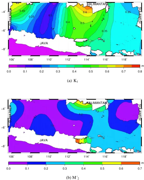
2.4.3 Tidal wave propagation

Tidal wave propagates westward in the Java Sea. M2 tidal wave is coming through the Flores Sea from the Indian Ocean while K1 tidal wave is coming through the Makassar Strait from the Pacific Ocean (Hatayama et al.

1996). Co-range and co-tidal charts of M2 and K1 constituents calculated by our model are shown in Fig.7 and Fig.8, respectively.

22

(a) K1

(b) M´2

Figure 7. Co-range charts of K1 and M´2 tidal amplitude (unit is meter)

23

(a) K1

(b) M2

Figure 8. Co-tidal charts of K1 and M2 tidal phase (unit is degrees referred to Indonesian mean time GMT+8 hours)

24

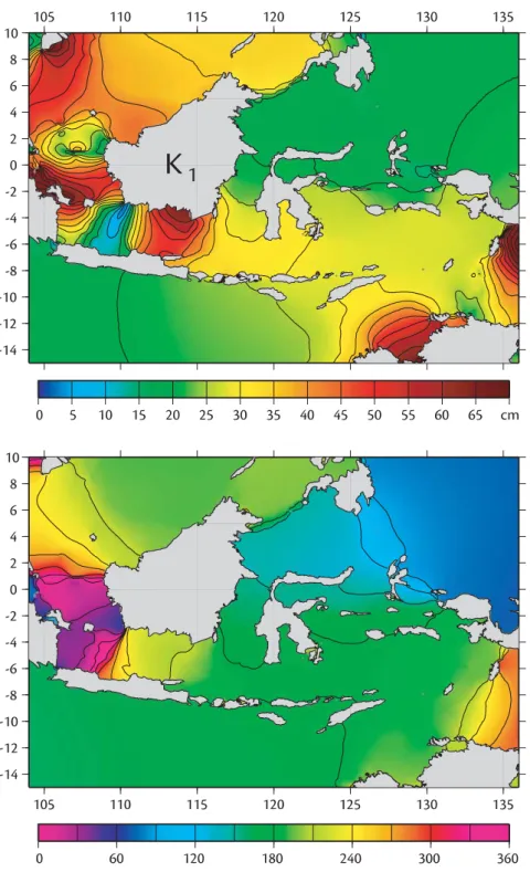
Figure 9. Co-range chart (upper figure) and co-tidal chart (lower figure) of K₁ tide in Indonesian Seas (after Ray, et all., 2005)

25

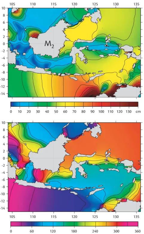
Figure 10. Co-range chart (upper figure) and co-tidal chart (lower figure) of M₂ tide in Indonesian Seas (after Ray, et all., 2005))

26

Model results show that there is counterclockwise phase propagation of M2 tidal wave in the Java Sea. The phase of tides is well known to propagate counterclockwise in the northern hemisphere and propagates clockwise in the southern hemisphere (Yanagi and Takao, 1998). In the case of the Java Sea which is located in the southern hemisphere but the phase of M2 tide propagates counterclockwise. The direction of the phase propagation is mainly governed by the large amplitude part of the incoming wave from the Flores Sea through the Makassar Strait. The large amplitude part propagates along the northern boundary (southern coast of Kalimantan Island). The same propagation type has been reported by Yanagi and Takao (1998) in the Gulf of Thailand which is located in the northern hemisphere but the semi-diurnal tide propagates clockwise, which is governed by the propagation of the large amplitude part of the incoming wave.

Diurnal tide (K1) as well as semi-diurnal tide (M2) propagates from the eastern part to the western part of the Java Sea.

It is clearly seen from the co-tidal charts (Fig.8) that tidal wave propagates faster in the central southern part of the Java Sea (off the central Java island) rather than the central northern part of the Java Sea (off the Kalimantan island) due to the bottom topography of the Java Sea, where the southern part is

27

deeper than the northern part. The bottom topography is also the reason of the difference of tidal amplitude distribution of K1 as well as M2 which are larger in the northern part rather than the southern part of the Java Sea (Fig.7).

It is also seen that M2 tide (Fig.8b) from the Indian Ocean and the Flores Sea bifurcates in the Makassar Strait, with one propagating into the Java Sea and the other continuing northwards to the northern part of the Makassar Strait. On the other hand, K1 tide propagates southward in the Makassar Strait and afterward it shifts into the Java Sea and continuing westwards to the western part of the Java Sea (Fig.8a). Model results also show that diurnal component propagates slower than semi-diurnal component. Since the natural oscillation period of the Java Sea is close to the period of K1 tide, so the reflected K1 tidal wave will resonate with the incoming wave. Hence, the resonance decreases the wave speed on the node in the central part of the Java Sea. It is seen from the dense line of K1 tidal phase on the co-tidal chart of K1 (Fig.8a). These results are similar to the previous authors, Ray et al. (2005) in Fig.9 and Fig.10, and Koropitan & Ikeda (2008). In the northern part of the Java Sea, the K1 and M2 tide will continue the propagation to the north entering the Karimata Strait and meet with the K1 and M2 tide from the South China Sea.

28

2.4.4 Tidal energy propagation

The previous authors (Ray, et al., 2005 and Zu, et al., 2008) have shown the tidal energy propagation in the Indonesian Seas for K1 and M2 tide. Ray, et al.

(2005) have found that the mean barotropic energy flux vectors for the K1 tide propagate southward in the Makassar Strait while those for the M2 tide propagate northward. Similar results are also shown by Zu, et al. (2008). However, they neglected the energy flux in the Java Sea in their diagram.

In the present study, calculated results of the COHERENS model are analyzed to obtain the tidal energy balance using the equation (2.15). In the transformed and vertically integrated form, the model equations are written as follow (Luyten, 2011),

𝜕

𝜕𝑡(𝐸̅̅̅ + 𝐸_{𝑘 𝑝}) +_ℎ¹

1ℎ₂[_𝜕𝜉^𝜕

1(ℎ₂𝐹̅ ) +_{1 𝜕𝜉}^𝜕

2(ℎ₁𝐹̅̅̅)] = 𝐷̅ (2.15) ₂

where 𝐸_𝑘

̅̅̅ =¹₂𝜌₀∫ ℎ𝑁_𝑧 3

0 (𝑢²+ 𝑣²)𝑑𝑠; 𝐸_𝑝= ¹₂𝜌₀𝑔𝜁² (𝐹̅ , 𝐹₁ ̅̅̅) = ∫ ℎ_{2 0}^𝑁𝑧 ₃[¹₂𝜌₀(𝑢²+ 𝑣²) + 𝜌₀𝑔𝜁](𝑢, 𝑣)𝑑𝑠

𝐷̅ = 𝜌₀(𝑢_𝑠𝜏_𝑠1+ 𝑣_𝑠𝜏_𝑠2− 𝑢_𝑏𝜏_𝑏1− 𝑣_𝑏𝜏_𝑏2) − 𝜌₀∫ 𝜐_𝑇 ℎ₃[(𝜕𝑢

𝜕𝑠)

2

+ (𝜕𝑣

𝜕𝑠)

2

]

𝑁_𝑧

0

𝑑𝑠

where 𝐸_𝑘 is the kinetic energy; 𝐸_𝑝 is the potential energy; D is the dissipation of

29

energy by turbulent diffusion; ℎ₁, ℎ₂, ℎ₃ is the grid spacing in the three (transformed) coordinate directions; 𝜉₁, 𝜉₂ is the orthogonal curviliniear coordinates. 𝐹₁, 𝐹₂ is the energy flux vector; (𝑢_𝑠, 𝑣_𝑠) and (𝑢_𝑏, 𝑣_𝑏) are the velocity respectively the surface and the bottom; (𝜏_𝑠1, 𝜏_𝑠2) and (𝜏_𝑏1, 𝜏_𝑏2) are the components of surface and bottom stress respectively; 𝜐_𝑇 is vertical viscosity coefficient.

30

(a) K1

(b) M´2

Figure 11. Depth-integrated energy flux vectors for K₁ and M´₂ tide during one tidal cycle

31

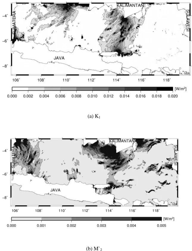
Our model results (Fig. 11) show that the energy flux vectors in the Makassar Strait are in accordance with the previous authors and we found that the tidal energy in the Java Sea propagates westward. It is clearly seen that the eastern part of the Java Sea is the inlet of the energy flux while the Sunda Strait is the outlet in the southern part as well as Karimata, Gaspar and Bangka are the outlet in the northern part. Energy flux vectors for the K1 tide that propagate southward in the Makassar Strait are shifted westward into the Java Sea. On the other hand, energy flux vectors for the M2 tide are partially shifted westward into the Java Sea.

K1 and M2 energy flux vectors indicate that the energy fluxes entering the Java Sea are coming from the Pacific Ocean and Indian Ocean. The loss of tidal energy while tidal waves entering the Java Sea, is indicated by the smaller magnitude of both K1 and M2 energy fluxes in the central part rather than those in the eastern part due to the steep bottom topography. Nevertheless, the magnitude of K1

energy flux in the western part is larger due to the amplification in accordance with K1 resonance period.

An interesting phenomenon appears in the Karimata Strait where Zu, et al. (2008) have described that K1 tidal energy flux vectors from the South China Sea propagate southward while our model result shows, in the northern part of the

32

Java Sea, that the K1 tidal energy flux vectors shift towards the Karimata Strait.

Our model result shows that the large K1 tidal energy dissipates on the southern tip of Karimata Strait (Fig. 12a). Nevertheless, the reason of the difference of ours and Zu et. al. (2008) needs more detail study.

The distribution of vertically integrated energy dissipation for K1 and M´2

tide in the Java Sea are shown in Fig.12. It is clearly seen that the tidal energy fluxes are dissipated in the inlet while entering the Java Sea. In contrast with the K1 tidal energy flux (Fig. 12a), the M2 tidal energy flux is dissipated in the western part of the Java Sea (Fig. 12b).

33

(a) K1

(b) M`2

Figure 12. Vertically integrated energy dissipation of K₁ and M´₂ tide during one tidal cycle

34

2.4.5 Tide-induced residual current

The information about the residual flow in the shelf seas is very important because it is related with long-term material transport in that area. Even though the velocity of tidal residual flow is smaller than the tidal current but it plays more important roles for the long-term material transport. This phenomenon has been pointed out by Yanagi (1974), Zimmerman (1978) and others as reported by Yanagi and Yoshikawa (1983).

The flow pattern of the tide-induced residual current in the Java Sea, has been reported by Koropitan & Ikeda (2008). Nevertheless, they found a very complicated residual flow pattern of K1 in the western part that is not agreed with the nature of tide-induced residual flow which forms a rotational flow pattern. The generation mechanisms of such rotational flow in relation to the tide-induced residual current have been described by Yanagi and Yoshikawa (1983) based on the previous result (Yanagi, 1976, 1978 and Oonishi, 1977).

35

Figure.13 Depth-mean tide-induced residual current generated by K₁ tide (after 5x5 grids box averaging). Upper figure shows the whole model area, lower figure shows more detail for the Java Sea

36

Figure.14 Depth-mean tide-induced residual current generated by M´₂ tide (after 5x5 grids box averaging). Upper figure shows the whole model area, lower figure shows more detail for the Java Sea

37

Fig.13 and Fig.14 show our model results for the tide-induced residual current in the Java Sea generated by the K1 and M2 tide, respectively. The tide-induced residual current generated by the K1 tide forms a counterclockwise rotational flow.

The rotational flow objectively determined by performing 5x5 grid box averaging.

The current flows westward in the northern part along the coast of Kalimantan and shifts to south in the western part along the east coast of Sumatera then shifts to east in the eastern part of the Java Sea along the north coast of Java, then shifts to north just when it reaches the Makassar Strait to complete the rotation. This flow pattern is formed due to geometrical boundary effect and bottom topography that correspond with the generation mechanisms described by Sugimoto (1975) and Yanagi & Yoshikawa (1983) in the Seto Inland Sea. Sugimoto (1975) has pointed out the effects of the coastal boundary geometries on tidal current and tidal mixing. The flows are bent under the kinematic and the dynamic restraints of the boundary. Residual circulations are produced by the non-linier effect of the flow patterns due to boundary geometries. Yanagi and Yoshikawa (1983) have shown the generation mechanisms of tidal residual flow related to the presence bottom slope and horizontal boundary. Tidal current deflects to the shallower part (northern part) to achieving the same tidal height because the shallower part has a

38

small tidal volume transport. The presence of horizontal boundary (southern part of Kalimantan Island) makes the current flows westward. Then, the flows are bent to the south in the north corner as well as bent to the east in the south corner owing to the boundary geometries (eastern part of Sumatera Island) in the western part of the Java Sea. Similar pattern is also shown by the M2 in the eastern part of the Java Sea, but a remarkable clockwise rotational flow appears in the western part. We suppose that the increasing of M2 tidal amplitude due to the shoaling effect and solid boundary generates this pattern.

39

2.4.6 Tidal fronts

It is well known that tidal front is generated in the shelf areas in summer, in a transition zone between vertically mixed water caused by tidal stirring and stratified water caused by heating through the sea surface (Yanagi and Koike, 1987). Tidal front in the shelf seas has already been studied by many authors (e.g.:

Simpson and Hunter, 1974; Yanagi and Koike, 1987; Yanagi and Takahashi, 1988).

Such tidal front coincides with the value of log(H/U³), where H is the water depth in m and U is the amplitude of tidal current in m s^-1, and known as ‘critical value’

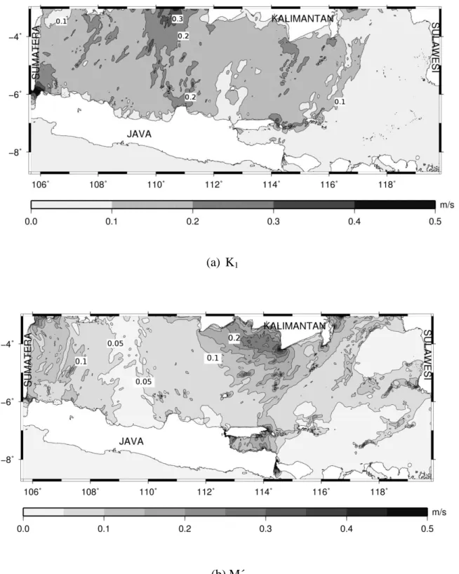
(Sun and Isobe, 2008). In the present study we calculate the log(H/U³) value using the velocity component of M´2+K1 to identify the tidal fronts in the Java Sea. The velocity component of M´2+K1 was chosen based on the horizontal distribution of tidal current amplitude shown in Fig.15.

40

(a) K1

(b) M´2

Figure 15. Co-range chart of K₁ and M´₂ tidal current amplitude

41

Fig.16 shows the isolines of the log(H/U³). A composite image of several satellite images from MODIS-Aqua 4km (4 micron night) on March year 2008, 2011 and MODIS-Tera 4km (4 micron night) on March year 2009 (Fig.17) shows the sea surface temperature distribution in the Java Sea. MODIS data used in this study were produced with the Giovanni online data system, developed and maintained by the NASA GES DISC (Acker and Leptoukh, 2007). The image shows the temperature front in the northern part of the Java Sea along the southern coast of Kalimantan as well as in the western part along the east coast of South Sumatera. Comparing the model result (Fig.16) and the satellite image (Fig.17), we found that the temperature front coincides with the 3.5 value of log(H/U³).

Thus, we conclude that the critical value for tidal front generation in the Java Sea is 3.5. This critical value is nearly the same with the results of previous authors (Yanagi and Koike, 1987; Yanagi and Takahashi, 1988) in Osaka Bay, Japan that is 2.5 – 3.0 of log(H/U³) and 3.0 – 3.5 of log(H/U³) in the absence of river discharge effect. This critical value means how strong the tidal current required to destroy the stratification. In the case of the Java Sea, the front is formed along the transition zone and separates the well-mixed nearshore region around Kalimantan Island from the stratified region of the center of the Java Sea.

42

Figure.16 Isoline of Log(H/U 3). White color denotes the value over than 4.5

43

Figure.17 Sea Surface Temperature distribution on nighttime of March, composite of MODIS-Aqua

4km (4 micron night) in year 2008, 2011 and MODIS-Tera 4km (4 micron night) in year 2009

images. White color on the sea indicates the clouds omission.

44

CHAPTER 3 Conclusions

In the present study we have shown that the K1 tide is coming from the Pacific Ocean while M2 tide is coming from the Indian Ocean. We have clearly shown the co-tidal and co-range charts of M2 and K1 tide, as well as the westward propagation of the K1 and M2 tides in the Java Sea in agreement with the previous studies, so we conclude that our model can reproduce well the tidal dynamics in the Java Sea.

Based on the facts above and according to our model results, we arrive at the new conclusions that the tidal energy flux propagates westward in the Java Sea where the magnitude is decreased after entering the inlet, indicating the large energy loss at the inlet. This finding suggests the importance of the existence of steep topography at the Java Sea inlet. Counterclockwise rotational flow of tide-induced residual current generated by the K1 tide is due to the boundary geometry and topography effect while the clockwise rotational flow by the M2

tide that appears in the western part is due to the bottom topography and shoaling effect. Tidal front is formed near the coastal water of Kalimantan. The critical

45

value is found to be 3.5 of log(H/U³), that is nearly the same with the values generally found in the other areas by the previous authors.

Based on the current results, we will examine more the consistency of the fronts by incorporating the wind driven current and the density driven current in the next study.