G-1. Japan area experiment to support T-PARC G-1-1. Overview and motivation
After the B08RDP experiment in 2008, the domain of the mesoscale ensemble prediction (MEP) system at MRI/JMA constructed for B08RDP (Fig. D-2-1) was shifted to cover Japan area (Fig. G-1-1) with some modifications, and then the new system was operated routinely in near-real time. The purpose of this experiment was to evaluate our MEP system for Japan region, where more observational data were available for its verification, and to support the THORPEX Pacific Asian Regional Campaign (T-PARC) experiment conducted around the same time. In addition to the execution of the MEP system, sensitivity analysis using mesoscale singular vectors (MSV) was tested.
In this section, preliminary results of the MEP experiment and the sensitivity analysis will be shown.
G-1-2. Experimental design and results
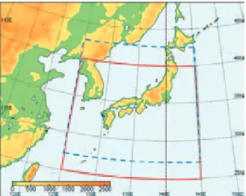
The experimental system used for the Japan area MEP experiment was almost the same as that for B08RDP. Specifications of the experiment are listed in Table G-1-1. The JMA mesoscale analysis was used for the initial condition, and therefore mesoscale analysis did not need to be performed at MRI separately, unlike B08RDP. The JMA nonhydrostatic model (NHM) was employed as the forecast model. Horizontal resolution was 15km and vertical resolution changed linearly from 40 m at the bottom to 1180 m at the top. For initial and lateral boundary perturbations, the global singular vector (GSV, T63L40) method was adapted in the same way of B08RDP. The optimization time used in GSVs calculation was 24 hours and the target area was set to the southern Japan region (25.0-40.0N, 125.0-145.0N; see Fig G-1-1). The number of ensemble member was 11, including the non-perturbed control run. The forecasts were performed once a day at 12 UTC.
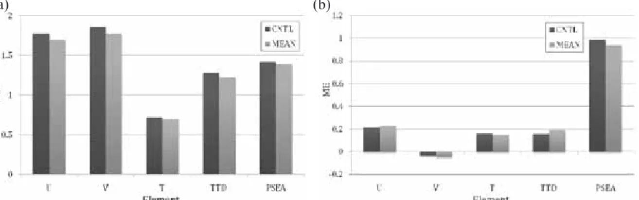
First, the averaged verification scores over the experimental period (1st – 26th September 2008) are shown. Figure G-1-2 shows RMSEs and MEs of a control run and the ensemble mean at FT=24 for variables at surface level against analysis field. RMSEs of the ensemble forecast were smaller than those of the deterministic forecast, which suggests that the ensemble system also performed well over Japan region. ROC diagram is illustrated in Fig. G-1-3.
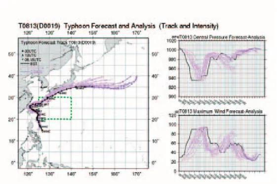
Next, we show some preliminary results of this EPS system applied to the case of Typhoon SINLAKU (2008). Figure G-1-4 shows the best-track of RSMC Tokyo - Typhoon Center, and the GSM forecast results for this typhoon. The typhoon generated at 18 UTC 8 September over the sea east of Philippine and moved northwestward while developing. Its minimum central pressure reached 935 hPa at 12 UTC 10 September. After landfall in the northern part of Taiwan, the typhoon moved northeastward and approached Japan. It brought torrential precipitation and strong winds while approaching, especially more than 700 mm per 24-hour rainfall was observed in the Tokai district.
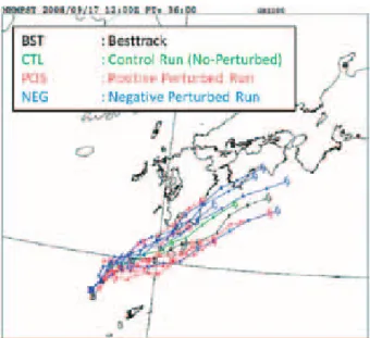
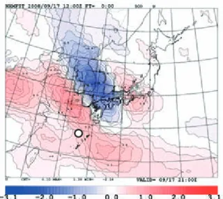
Figure G-1-5 shows variations of ensemble spreads and the comparison of RSMEs between the control forecast and ensemble mean, initialized at 12 UTC on 17 September 2008. We can see the steady growth of spreads through the forecast period, which seemed to be comparable with the standard forecast errors. Besides, the RMSEs of ensemble mean outperformed those of the control forecast. The forecasted typhoon tracks are illustrated in Fig. G-1-6. Although the track of the control forecast was a bit slower than the best-track, some members successfully reduced the error, which was obvious for the negative-perturbed members. Figure G-1-7 shows track errors and simulated central pressures of all members. The most notable characteristic from the result was that the
negative-perturbed members ameliorated the intensity as well as the track forecast of the typhoon.
Figure G-1-8 illustrates the perturbation field of zonal wind at 500 hPa of member m04. We can infer from the figure that the west-wind perturbation spreading west of the typhoon contributed for the amelioration of track error of the control forecast. These results indicate a great potential of mesoscale EPS for typhoon forecasts.
G-1-3. Sensitivity Analysis
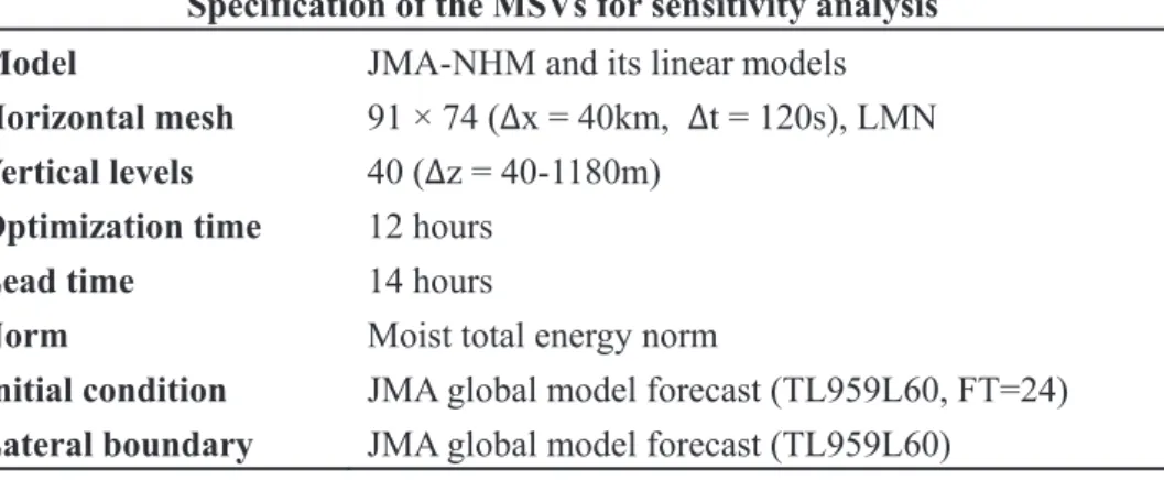
In addition to the EPS experiment, we performed sensitivity analysis using MSV. The domain and target area of the experiment is shown in Fig. G-1-1. Specifications of the MSV for the sensitivity analysis experiment are summarized in Table G-1-2. Note that, for the near-real time operation, the 24-hour forecast of the JMA Global Spectral model (GSM; TL959L60) was used for the initial condition to calculate MSVs, so that lead time of about 14 hours was kept prior to the observation time of T-PARC.
Figure G-1-9a shows the vertically integrated initial total energy of 1st MSV normalized by the maximum value of total energy in the domain. The figure indicates the sensitivity area for the observational time (valid time). The horizontal scale of it was as large as 500 km, which was much smaller than that calculated using the dry model instead of one with moisture processes in linear model of NHM (Fig. G-1-9b). This dry experiment was carried out after the experimental period to examine the effect of moist processes on the sensitivity area. It seemed that the sensitivity area calculated by the moist linear model was effective for the intensity related to the cumulus convection around the typhoon while the area of dry model had an influence on the typhoon track if the initial field was modified dynamically through the data assimilation process with special soundings.
In order to assess the propriety of the MSV-based sensitivity region, OSSE on water vapor fields around typhoon center is necessary.
Fig. G-1-1. Model domain and target area for GSV (solid) and MSV (dash).
Fig. G-1-2. (a) RMSEs and (b) MEs (FT=24) against analysis fields at surface level, averaged from 1st to 26th Septenber 2008.
Fig. G-1-3. ROC area skill score averaged from 1st to 26th Septenber 2008.
(a) (b)
Fig. G-1-4. Track and intensity of typhoon SINLAKU. Black line and purple line indicate best-track data forecast results by the GSM, respectively.
Fig. G-1-5. (a) Variations of ensemble spreads of surface elements and (b) the comparison of RMSEs
between a control forecast and ensemble mean.
(a) (b)
Fig. G-1-6. Best-track (blue) and forecasted typhoon tracks (colors) for SINLAKU. Initial time of the experiment was 12 UTC on 17 September 2008.
Fig. G-1-7. (a) Track error and (b) variations of central pressure simulated by all members. Blue lines indicate positive-perturbed members, and red lines indicate negative-perturbed members.
(a) (b)
Fig. G-1-8. Perturbation field of zonal wind at 500 hPa of member m04 at 12 UTC on 17 September 2008.
Open circle denotes the typhoon center derived from the control forecast.
Fig. G-1-9. Vertically integrated initial energy norm of 1st MSV at 12 UTC on 18 September 2008 calculated by the linear model of NHM (a) with (b) without moist processes.
(a) (b)
Table G-1-1. Specification of the Ensemble Forecast over Japan area Specification of the Ensemble Forecast over Japan area Numerical model JMA-NHM as of July 2008
Horizontal mesh 239 × 191 (∆x = 15km, ∆t = 60s), LMN Vertical levels 40 (∆z = 40-1180m)
Forecast period 36 hours
Member 11 (= control run + 10 perturbed runs)
Initial condition The JMA meso 4D-Var + NHM 3hour forecast Lateral boundary The JMA global model forecast (TL959L60) Initial perturbation Targeted moist global SV (T63L40)
Lateral perturbation Forecast of global model initiated by targeted SV
Table G-1-2. Specification of the MSV for the sensitivity analysis experiment.
Specification of the MSVs for sensitivity analysis Model JMA-NHM and its linear models Horizontal mesh 91 × 74 (∆x = 40km, ∆t = 120s), LMN Vertical levels 40 (∆z = 40-1180m)
Optimization time 12 hours
Lead time 14 hours
Norm Moist total energy norm
Initial condition JMA global model forecast (TL959L60, FT=24) Lateral boundary JMA global model forecast (TL959L60)
G-2. Heavy rainfall experiments
G-2-1. Heavy rainfall experiments using mesoscale SV
We examined a heavy rainfall event that occurred in August 2008 in Japan to investigate the characteristics of MSVs and to assess the subsequent ensemble forecast as probabilistic information.
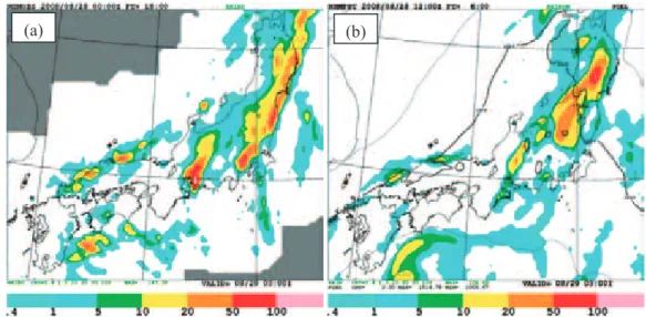
On 29 August 2008, a torrential rainfall occurred over the Tokai and Kanto districts, and a maximum cumulative hourly rainfall of 144 mm was recorded at Okazaki City. Horizontal distributions of the 3-hour cumulative analyzed rainfall (interpolated into a model with a grid interval of 15 km) and that predicted by the control forecast at 18 UTC on 28 August 2008 are shown in Fig. G-2-1. The control forecast failed to capture the rainfall. Therefore, we applied the MSV-based mesoscale EPS to this event and evaluated its potential to produce a probabilistic forecast.
Figure G-2-2 shows the horizontal distributions of the vertically integrated initial energy of the MSVs. The second, third, and fifth leading singular vectors had high sensitivity over the Tokai district, where severe rainfall was observed 6 hours after the initial time. The MSVs were dominated in large part by the moisture term and captured small-scale structures, which affect mesoscale disturbances occurring over a short time span rather than synoptic events.
Ensemble forecast results are shown in Fig. G-2-3 as probabilities. The probabilistic values were normalized from 0 to 1 and were determined by the proportion of members that predicted precipitation above a certain threshold. The results generally captured the intense rainfall observed in the Tokai district well. The most notable characteristic was that a more than 30% probability of precipitation was estimated even with a large threshold of 50 mm/3 hours, whereas the control forecast predicted a rainfall of only about 20 mm/3 hours. When singular vectors are used as initial perturbations in ensemble predictions, a pair of perturbations with opposite signs is produced to keep the ensemble mean unbiased at the initial time. Therefore, the probability that a specific phenomenon happens cannot exceed 50% if the control forecast fails to capture the occurrence of the phenomenon. These results indicate that MEP with MSV appropriately compensated for the insufficiency of the control run, and reproduced well the conspicuous mesoscale disturbance.
Fig. G-2-1. Three-hour accumulated precipitation at 18 UTC on 28 August 2008. (a) Analyzed rainfall and (b) predicted rainfall by the control forecast (FT = 06).
(a) (b)
Fig. G-2-2. Horizontal distributions of vertically integrated initial energy of the MSVs at 12 UTC on 28 July 2008. Each value was normalized to a value from 0 to 1. (a) First, (b) second, (c) third, (d) fourth, and (e) fifth leading SVs.
Fig. G-2-3. Probability forecasts of 3-hour cumulative precipitation using MSVs for threshold values of (a) 20 mm and (b) 50 mm.
(a) (b) (c)
(d) (e)
(a) (b)
G-2-2. Heavy rainfall experiments using the local ensemble transform Kalman filter (LETKF)
Heavy rainfalls sometimes occur in Japan when the Baiu front stays over Japan or when a typhoon is south of Japan. Numerical simulations have been performed by deterministic forecasts so far to reproduce these heavy rainfalls. However, they are not always reproduced due to insufficient accuracy of either the initial conditions or the numerical models. The B08RDP experiment is the first international intercomparison of mesoscale ensemble forecasts. Because ensemble forecasts provide many scenarios of atmospheric conditions, some can reproduce the heavy rainfalls even when a deterministic forecast fails to reproduce them. Therefore, the miss rate of forecasts is expected to decrease when ensemble forecasts are used. An ensemble forecast can also give the probability of a heavy rainfall. In addition to these advantages, many numerical forecasts provide other useful information (e.g., the factors that cause the heavy rainfall). In this section, an ensemble forecast system using LETKF was applied to several heavy rainfall events that occurred in 2008: (1) the Oki intense rainfall, (2) the Okazaki heavy rainfall, and (3) the Kobe heavy rainfall. The procedures that can extract the factors leading to the heavy rainfall are explained in this subsection.
Before we present our results, we explain the ensemble forecast system. The Japan area mesoscale ensemble system used here is based on the local ensemble transform Kalman filter developed for B08RDP. Because many observation data are available in and around Japan, horizontal grid interval of LETKF system was set to 20 km. Assimilation data for operational mesoscale analysis (MA) and operational global analysis (GA) that passed the quality control procedures of these analysis systems were used. The boundary conditions of LETKF system were not perturbed, and the ensemble means were replaced with JMA operational Meso-4DVar analysis results each day at 12 UTC. The assimilation cycle was started two-three days before the occurrence of the heavy rainfall. The domain of LETKF system is roughly the same as that of the JMA mesoscale model, which covers Japan and the surrounding area. After the forecast-analysis cycles, extended forecasts were performed from the analyses obtained by LETKF without replacing the ensemble mean with Meso-4DVar analysis data.
The boundary conditions of the extended forecast were obtained from the JMA regional model.
Downscale experiments with horizontal grid intervals of 5 km and 1.6 km were also conducted. The initial and boundary conditions of the downscale experiments were produced by the extended forecast and the numerical forecast output with a grid interval of 5 km, respectively. The domain of downscale experiment with a 5-km grid interval covers all of Japan except for Hokkaido, and the 1.6-km grid interval domain covers those few districts where the heavy rainfall occurred. Because the boundary conditions of the LETKF system were not perturbed, their influence moves inward during the numerical integrations. Thus, the results of downscale experiments in the region far from the boundary of the LETKF domain are mainly discussed in this section.
a) Oki intense rainfall
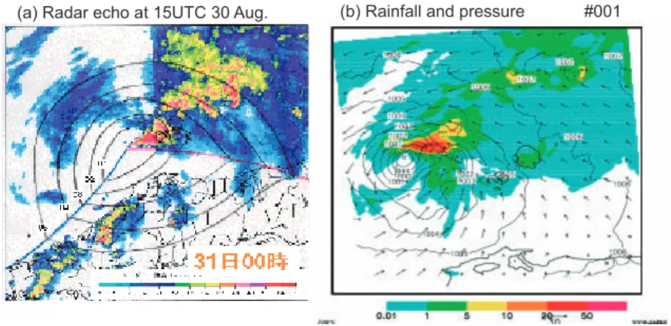
Figure G-2-4a shows the weather chart at 12 UTC on 31 August 2007 for the region of the Oki Islands. A low-pressure system, which was changed from a tropical depression, was north of western Japan. A stationary front extended from west to east through the center of the low-pressure system.
Associated with this low-pressure system, a rainfall system in which the rainfall intensity exceeded 80 mm/hour was developed (Fig. G-2-4b). This rainfall system developed abruptly as the system moved
eastward, causing the heavy rainfall over the Oki Islands. When this system passed the Oki Islands, abrupt change of wind directions of strong winds and a sharp drop in surface pressure were observed (Fig. G-2-4c).
The MA and GA data (designated ‘cda’ in the JMA operational numerical weather prediction system) were assimilated by using LETKF system. The assimilation cycles reproduced this intense rainfall north of western Japan. Because fewer assimilation data were available over the sea, ensemble spreads over the sea were larger than those over the land (not shown). Near the rainfall system in particular, large variation of the position and intensity of the low-pressure system caused the ensemble spread to be larger. Although the positions of the rainfall system produced by the ensemble members were scattered, one ensemble member of the downscale experiment using a non-hydrostatic model (NHM) with the horizontal grid interval of 5 km reproduced the rainfall system at the position where it was actually observed.
Downscale experiment of the member in which the position of the rainfall system was well reproduced was further performed using the NHM with a grid interval of 1.6 km. Figure G-2-5 shows the rainfall region reproduced by this experiment. The reproduced rainfall system had a triangular shape, and a low-pressure system was also reproduced at the southwestern edge of the rainfall region.
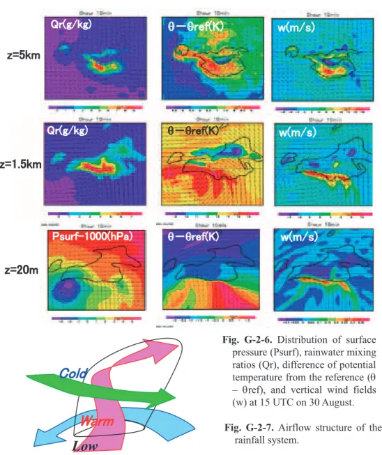
Several features, such as the scale and shape of the rainfall system, the rainfall intensity, and the pressure distribution, were similar to the observed features. Since the rainfall system was reproduced well, the structure of the heavy rainfall was investigated (Figs. G-2-6 and G-2-7). The rainfall system
(c)Temporal variation of pressure (b) Radar echo at 15UTC 30 Aug.
(a) Weather chart at12UTC 30 Aug.
(a) Radar echo at 15UTC 30 Aug. (b) Rainfall and pressure #001
Fig. G-2-4. (a) Weather chart at 12 UTC on 30 August 2007. (b) Radar echo distribution at 15 UTC on 30 August. (c) Temporal variation of pressure observed at Saigo in the Oki Islands. Red arrow indicates the Oki intense rainfall.
Fig. G-2-5. (a) Radar reflectivity at 15 UTC on 30 August, and (b) rainfall (arrows) and pressure distribution (contours) at 15 UTC on 30 August as reproduced by ensemble member #001.
16 17 18 19 20 (UTC)
was composed of the following 3 airflows. A southerly airflow near the surface was converged with the easterly flow on the northern side of the system, and then ascended. A low-level warm air mass around the southwestern tip of the rainfall region produced the sharp drop in pressure. When a cold airflow at the mid-level approached the rainfall region, the convections developed. It is deduced that the development of the convection reinforced the intensity of vorticity.
b) Okazaki heavy rainfall
Figure G-2-8 shows the weather chart and 3-hour rainfall at 15 UTC on 28 August 2008 around Okazaki. A stationary front extended along Japan (Fig. G-2-8a). On the southern side of the front, a few rainfall systems that extended from south to north were organized in central Japan. The Okazaki heavy rainfall was caused by one of these rainfall bands (indicated by a red arrow in Fig. G-2-8b). The record-breaking rainfall, a 1-hour rainfall of 146.5 mm, was brought by this rainfall system, which was maintained by a southerly airflow. This southerly airflow was produced by the presence of a low-pressure system south of western Japan and a high-pressure system east of Japan. Southerly airflow produced by low- and high-pressure systems acts as conveyor belt that carries warm and
Qr(g/kg) θ-θref(K) w(m/s)
z=5km
z=1.5km
Qr(g/kg) θ-θref(K) w(m/s)
θ-θref(K) w(m/s) Psurf-1000(hPa)
z=20m
Fig. G-2-6. Distribution of surface pressure (Psurf), rainwater mixing ratios (Qr), difference of potential temperature from the reference (θ – θref), and vertical wind fields (w) at 15 UTC on 30 August.
Low Warm Cold
Fig. G-2-7. Airflow structure of the rainfall system.
humid air, and then causes heavy rainfall over Okazaki. The JMA operational numerical weather prediction (NWP) system was able to forecast this rainfall system using its mesoscale model when the initial conditions at 00 UTC or 03 UTC were used. However, the rainfall system was not reproduced when the initial conditions after 06 UTC were used.
Figure G-2-9 shows the analysis results. Rainfall corresponding to the observed heavy rainfall was well reproduced by most ensemble members (Fig. G-2-9c). Because the ensemble mean was replaced with the analyzed fields of the Meso-4DVar analyses every day at 12 UTC, accurate Meso-4DVar analysis data could enable this high
probability of heavy rainfall, though the analysis of the Meso-4DVar after 06 UTC could not reproduce the heavy rainfall. The southeasterly airflow into the rainfall system, between the low-pressure region south of western Japan and the high-pressure east of Japan, was also reproduced (Fig. G-2-9a). The ensemble spread of horizontal wind south of Japan was relatively large (Fig. G-2-9b), and this large spread affected the rainfall amount and duration of the predicted heavy rainfall.
Spaghetti diagrams showing the contour lines for some threshold values or the horizontal wind vectors of all members are plotted in Fig.
G-2-10. All ensemble members reproduced the southeasterly flows between the low-pressure system south of western Japan and the high-pressure system east of Japan.
The reproduced wind speeds at a few hundreds of kilometers south of Japan varied greatly among ensemble members, though the spread of wind speeds near Japan was small. As mentioned in relation to Fig. G-2-9b, this large variation in horizontal winds can affect the forecasted duration of the heavy rainfall. Water vapor and temperature were not very different
(a) Weather chart
15UTC 28 (b) Observation
12-15UTC 28
Fig. G-2-8. (a) Weather chart and (b) 3-hour rainfall at 15 UTC on 28 August 2008. Red arrow indicates the rainfall system that caused Okazaki heavy rainfall.
(a) Mean 12-15 UTC 28 (b) Spread 12-15 UTC 28
Fig. G-2-9. (a) Ensemble mean and (b) spread at 15 UTC on 28 August 2008 as reproduced by LETKF. (c) Analyzed rainfall fields obtained by LETKF.
#000 #001 #002
#003 #004 #005
(c) Analyzed fields 12-15 UTC 28
among the ensemble members, as all members reproduced the warm, humid southerly airflow to Japan.
Because the cold air mass overlaid the low-level warm humid airflow in all ensemble members, the atmospheric condition over central Japan was favorable to the generation and development of convections. As a result, the heavy rainfall was reproduced by most ensemble members.
When the downscale experiment was performed, differences appeared among the ensemble members. The contours in Fig. G-2-11a indicate the regions where the 1-hour rainfall amount exceeded 5 mm. In the ensemble
member #002 result, the rainfall region became smaller as the system moved northeastward, whereas in the #005 result, it remained large. What factors caused this difference in the heavy rainfall between these ensemble members? We determined the factors that affected the rainfall amount by the following procedures. (1) The average 1-hour rainfall amount at 23 UTC on 29 August within the blue square in Fig.
G-2-11a that includes Okazaki was obtained from the ensemble forecast results. (2) The averages of the variables expected to affect rainfall intensity were also obtained from the ensemble
0.1 5.1 0.1
5.6 0.2 0.7
0.7 1.4
0.1 1.9 3.20.3
1.4 1.5 0.4 5.5 0.1
2.7 6.5
24.6 24.8 25 25.2 25.4 25.6
357.5 358 358.5 359 359.5 360
T (1000hPa)
5.5 0.1 5.1
0.1 5.6 0.7 6.5
0.20.7 2.7 1.4
0.1 1.9
0.3 1.43.2
0.4 1.5
0.1 0.0025
0.0027 0.0029 0.0031 0.0033 0.0035
0.0216 0.0218 0.022 0.0222 0.0224 0.0226
Qv(500hPa)
5.5 5.1 0.1
0.1 5.6 6.5
0.7 0.2
0.7
1.4 2.7
0.11.9
0.3 3.2
1.4
1.5 0.4 0.1
-0.8 -0.6 -0.4 -0.2 0 0.2 0.4 0.6
0.021 6
0.021 8
0.022 0.022 2
0.022 4
0.022 6
y = 0.0015x - 0.004
-0.015 -0.01 -0.005 0 0.005 0.01
0 2 4 6 8
Qv(1000hPa)
V (1000hPa) Qv*V(1000hPa)
θe(1000hPa)
1-hour rainfall
#002 #005
#005
#002
#005
#002
Qv (1000hPa) 0.1 5.1
0.1 5.6 0.2 0.7
0.7 1.4
0.1 1.9 3.20.3
1.4 1.5 0.4 5.5 0.1
2.7 6.5
24.6 24.8 25 25.2 25.4 25.6
357.5 358 358.5 359 359.5 360
T (1000hPa)
5.5 0.1 5.1
0.1 5.6 0.7 6.5
0.20.7 2.7 1.4
0.1 1.9
0.3 1.43.2
0.4 1.5
0.1 0.0025
0.0027 0.0029 0.0031 0.0033 0.0035
0.0216 0.0218 0.022 0.0222 0.0224 0.0226
Qv(500hPa)
5.5 5.1 0.1
0.1 5.6 6.5
0.7 0.2
0.7
1.4 2.7
0.11.9
0.3 3.2
1.4
1.5 0.4 0.1
-0.8 -0.6 -0.4 -0.2 0 0.2 0.4 0.6
0.021 6
0.021 8
0.022 0.022 2
0.022 4
0.022 6
y = 0.0015x - 0.004
-0.015 -0.01 -0.005 0 0.005 0.01
0 2 4 6 8
Qv(1000hPa)
V (1000hPa) Qv*V(1000hPa)
θe(1000hPa)
1-hour rainfall
#002 #005
#005
#002
#005
#002
Qv (1000hPa)
#005
#002
#005
#002
#005
#005
#002 (a)
(b)
(c) (d)
(e) (f)
Fig. G-2-11. Regions where the 1-hour rainfall exceeded 5 mm in the results of ensemble members (a) #002 and (b) #005. (c)–(e) Scatter diagrams of the variables expected to affect the occurrence of heavy rainfall. The size of the circles indicates the relative intensity of the 1-hour rainfall. (f) The product of the low-level water vapor and the speed of the southerly wind flow in relation to the 1-hour rainfall.
K=2、Qv=0.019
K=2、PT=300
W
Wet K=10 (1.2km)
K=18(4.2km)、PT=277 C
W
K=2、Qv=0.019
K=2、PT=300
W
Wet K=10 (1.2km)
K=18(4.2km)、PT=277 C
W
Fig. G-2-10. Spaghetti diagrams of low-level horizontal wind, water vapor, and temperature near the surface, and mid-level temperature.
K=2(20m), T=300K K=18(4.2km), T=277K K=2(1.2km) K=2(20m), Qv=0.019kg/kg
Warm Warm
Cold
forecast results. Specifically, the average of low-level temperature and water vapor and the southerly wind velocity within the red rectangle, which exists south of the blue square, were also obtained. (3) Scatter diagrams of the 1-hour rainfall amount and of the variables expected to affect rainfall amount were plotted. In the case of a variable that greatly affects the rainfall amount, intense and weak rainfalls should have separate distributions on the diagram. Figures G-2-11c–e show the scatter diagrams for temperature, water vapor, and southerly wind velocity. Large rainfall amount was obtained when the low-level water vapor exceeded 22.2 g/kg (Fig. G-2-11d), but the influence of low-level temperature on the rainfall amount was apparently small, because a large rainfall amount was not produced even when the temperature was close to the maximum value among ensemble members (e.g., #002 in Fig. G-2-11c). The influence of the mid-level water vapor was also small, because its value ranged widely from 2.8 to 3.1 g/kg when the rainfall amount exceeded 5 mm/hour. In comparison with the temperature and water vapor, the southerly wind influence is clear: a large rainfall amount was not produced when northerly winds prevailed in the red region south of Okazaki (Fig.
G-2-11e). The 1-hour rainfall amount and the product of the water vapor mixing ratio and the velocity of the southerly airflow near the surface were positively correlated (Fig. G-2-11f), indicating that the rainfall amount was greatly influenced by the water vapor flux from the south in the lower atmosphere.
These findings show that the ensemble forecast results are useful for ascertain the mechanisms causing heavy rainfall.
c) Kobe heavy rainfall1
The operational assimilation data, that is, MA and GA data were used in the aforementioned experiments. In this experiment, a heavy rainfall event that occurred at Kobe on 28 July 2008 was reproduced with LETKF system by assimilation of GPS-derived precipitable water vapor (GPS-PWV) data.
Figure G-2-12a shows the surface weather chart at 00 UTC on 28 July 2008. Low-level airflow in the East China Sea passed around western Japan, supplying warm humid air to rainfall systems developed along the Baiu front (indicated by a red arrow in Fig. G-2-12a). A mid-level cold air mass expanded over western Japan (indicated by a blue line in Fig. G-2-12a). These distributions suggest that the atmosphere over western Japan was very unstable. Figure G-2-12b shows the rainfall intensity observed by the JMA operational radar. Two rainfall bands (indicated by a red arrow in Fig. G-2-12b) were generated along the northern
coastline of western Japan and near Kobe. A rapid rise of a local river in Kobe due to the heavy rainfall caused by the southern rainfall band claimed the lives of five people. Because this intense rainfall band was not reproduced when the MA and GA data were
1 This subsection was a digest based on Seko et al. (2010).
(b)
(850hPa)
-6℃
(500hPa) (a)
Kobe
Fig. G-2-12. (a) Surface weather map at 00 UTC on 28 July 2008. (b) Rainfall intensity observed by JMA operational radar at 05 UTC on 28 July 2008.
used as assimilation data, GPS-PWV data were added to the assimilation data. First, the intermediate profiles of relative humidity were produced from the PWV data and the statistical data that were obtained from outputs of ensemble forecast, and then the intermediate profiles were assimilated by LETKF system. Procedures for assimilation of GPS-PWV data were as follows. (1) GPS-PWV data from GPS receivers at heights within 100 m of the model topographic height were used. The effect of height differences between GPS sites and the model topography was adjusted by using the observed surface pressure and the water vapor mixing ratio, which were estimated by interpolation of meteorological observatory data. (2) Vertical profiles of the ensemble mean and spread of temperature and relative humidity were obtained from the ensemble forecast output. Relative humidity profiles of the ensemble mean were averaged over the region within ±100 km of the GPS sites. This averaged profile was used as the first guess profile. Profiles of the maximum spread of relative humidity over the same region were also obtained. Average and maximum profiles were used in this study so that the position errors of the convective band should be considered. (3) We assumed that the difference between the analysis data and the first guess data is proportional to the maximum spread. The intermediate LETKF profiles were produced by distributing the difference between the observed GPS-PWV and first guess PWV (the vertical sum of the first guess profile) to the values at the model layers on the basis of this assumption.
Figure G-2-13a shows a scatter diagram of the observed GPS-PWV and the first guess PWV.
GPS-PWV values were larger than the first guess values. Thus, assimilation of GPS-PWV data should result in intensification of rainfall. Examples of the first guess and intermediate profiles are shown in Fig. G-2-13b. Though the difference in relative humidity between the first guess and intermediate profiles appears to be large at higher layers, the difference in the water vapor amount is very small.
Figure G-2-14 shows the impact of GPS-PWV data. When GPS-PWV data were added to the assimilation data, the region of weak rainfall near Kobe (red circles) became wider. Thus, downscale experiments were performed with the NHM at grid intervals of 5 and 1.6 km. Figure G-2-15 shows the rainfall distributions reproduced by the downscale experiments. Because the water vapor distribution
Height(km)
RH(%)
20 40 60 80
20 40 60 80
PWV(mm)
First guess
Observation.
20 25 30 35 40 45 50
120 125 130 135 140 145 150
Red points are plotted
First guess Input
Height(km)
RH(%)
20 40 60 80
20 40 60 80
PWV(mm)
First guess
Observation.
20 25 30 35 40 45 50
120 125 130 135 140 145 150
Red points are plotted
First guess Input
Fig. G-2-13. (a) Scatter diagram of observed GPS-PWV and first guess PWV. (b) Example profiles of the intermediate data produced from the GPS-PWV and first guess of the ensemble forecast. The inset map shows the positions of the GPS-PWV data used in this study. First guess and intermediate profiles at red points on the map were plotted.
(a) (b)
was improved (not shown), the rainfall region and intensity became closer to the observed ones. The rainfall band near Kobe, but not the northern rainfall band, was reproduced by ensemble member #001.
This result suggests that the reproduction of water vapor north of Japan, which affected the northern band, was not improved by GPS-PWV data, because the GPS sites are located in Japan. Data from a wider area, such as GPS-PWV data from China and Korea or water vapor data over the sea observed by satellites, are needed to reproduce the northern rainfall band.
The factors that caused the heavy rainfall were investigated by the same procedure that was used to investigate the Okazaki heavy rainfall, except that the variables that were expected to influence the rainfall amount were changed to those that corresponded to the observation data. In this heavy rainfall case, surface and upper level sounding data from Yonago (indicated by a blue square in Fig. G-2-16a), Tomogashima (green square), and Kobe (red square) were chosen as the variables corresponding to the observation data.
The separation ratio between intense and weak rainfalls was calculated by as follows. (1) Ensemble GPS-PWV
w/o GPS-PWV (b) with GPS-PWV (a) w/o GPS-PWV
01UTC:#001 02UTC:#001 03UTC:#001
2.0UTC:#001 2.5UTC:#001 3.0UTC:#001
3.5UTC:#001
(a) 5km-NHM Init : 00UTC 28
Fig. G-2-14. (a) Ensemble mean of the 6-hour rainfall (color scale) and sea surface pressure (contours) when MA and GA data were assimilated.
(b) Same as (a) except for when MA data, GA data, and GPS-PWV data were assimilated.
Fig. G-2-15. (a) Rainfall distributions obtained in downscale experiments by member #001 using NHM with grid intervals of (a) 5 km and (b) 1.6 km. Rainfall intensity in (b) corresponds to the 1-hour rainfall (the 10-minute rainfall multiplied by 6).
(b) 1.6km-NHM Init : 00UTC 28
members producing the three highest and three lowest 1-hour rainfalls at Kobe (indicated by a red square in Fig. G-2-16a) were chosen. These members are referred to as the top and bottom members.
(2) In the estimation of the distances between members, differences of variables were normalized by their standard deviations. Distances of the variables among top and bottom members, and that between top and bottom members, were estimated as follows (Fig. G-2-16b);
where A and B are the combination of top or bottom members used. If A and B are set to the top members, then DAB is the distance among the top members. When A and B are set to the top members and the bottom members, DAB is the distance between top members and bottom members. v1 and v2 are the variables that were investigated, and σ is their standard deviation. (3) The separation ratio is defined as the distance between the top and bottom members divided by the sum of the distance among the top members and that among the bottom members. The separation ratio equation is thus
Figure G-2-16c shows the separation ratio matrix. Scatter diagrams with large and small separation ratios are shown in Fig. G-2-17. In this heavy rainfall case, the temperature at the height of 500 hPa above Yonago was a key factor influencing the rainfall amount near Kobe. By having such information available in advance, forecasters can concentrate on monitoring those observation data that are
) 2 2 ( .
, ,
, − −
= + G
D D
R D
Bottom Bottom Top
Top
Bottom Top
( ) ( )
, ( 2 1)3 1
3
1 2
2 2 2 2 21
2 1 1
, − − −
− +
=
∑ ∑
= =
v G v v
D v
A B
B A B
A
i i v
i i v
i i B
A σ σ
301.3 301.4 301.5 301.6 301.7 301.8 301.9 302 302.1 302.2
301 301.5 302 302.5
Kobe Yonago Tomogashima 01 02
UTC 0304
Rain, U_surf, V_surf ,θe_surf,θe_500hPa, T_surf, T_500hPa,θe_surf-θe_500hPa, T_surf-T_500hPa,
Kobe Yonago Tomogashima 01 02
UTC 0304
Rain, U_surf, V_surf ,θe_surf,θe_500hPa, T_surf, T_500hPa,θe_surf-θe_500hPa, T_surf-T_500hPa,
Fig. G-2-16. (a) Locations of averaging areas: Blue square: Yonago, Red square: Kobe; Green square: Tomogashima. (b) Schematic illustration of the distances of top and bottom three members. Sizes of circles indicate the 1-hour rainfall averaged over the red square. Lines are the distances estimated by Eq. G-2-2. Red, blue and yellow lines are the distances among the top three members, among the bottom three members and between top and bottom members, respectively. (c) The separation ratio matrix. Horizontal and vertical axes are the variables that are expected to affect rainfall amount.
(b)
(a) (c)
expected to most influence the rainfall amount. This idea that was proposed here is a new application of the ensemble forecast.
Fig. G-2-17. Example scatter diagrams of large and small separation ratios. Sizes of circles and indexes near the circles indicate the 1-hour rainfall amount averaged over the green square. Circle size of 0.0012 was multiplied by 20 to show their positions.
Ratio=1.15
265 265.5 266 266.5 267
300.75 301.25 301.75 302.25 302.75
-3 -2.5 -2 -1.5 -1 -0.5 0 0.5 1 1.5
-5 -4 -3 -2 -1 0 1
1.89 1.34 1.27
0.0437 0.0862 0.0012
Ratio=1.52
Kobe 03UTC T_surf (K) Yonago 01UTC V_surf (m/s)
0.0012 1.34 1.27 1.89
0.0862
0.0437
Ratio=0.98
G-3 Experiments on the potential parameters of tornado outbreak using ensemble techniques1
A tornado measuring 2 on the Fujita scale (Fujita, 1971) occurred in Nobeoka, Miyazaki on 17 Sep.
2006, derailing the limited express train and collapsing more than one thousand houses. On 7Nov.
2006, 9 people were killed and 26 people were injured by another tornado measuring 3 with the Fujita scale, which occurred in Saroma, Hokkaido. The structure and formation mechanisms of the tornados have been investigated in many context using cloud-resolving models (e.g. Mashiko, 2007; Kato 2007).
Collaborating with the Japan Meteorological Agency, the Meteorological Research Institute participated in the WWRP Beijing 2008 project (hereinafter, B08), and developed an ensemble forecast system for mesoscale events. In order to identify some potential parameters to estimate the tornado outbreak, the ensemble forecast system is applied to tornado forecasting for the Nobeoka and Saroma tornado cases. This section describes the specifications of the experiments and the results of the numerical simulations.
a) Specifications of the experiments
The numerical model and the method to generate the initial perturbations are the same as those in the 2006 preliminary experiment of B08. The model domain is set to be 3300 km x 3000 km in the zonal and meridional direction, respectively. The horizontal grid interval is 15 km. The ensemble initial conditions are produced by adding the normalized perturbations of one-week ensemble of JMA to the initial field of the JMA regional spectrum model (RSM) (Saito et al, 2006).
An ensemble forecast is performed for each tornado case; Nobeoka and Saroma tornado. The initial time of the ensemble forecast is 12 UTC of the previous day of the tornado outbreak for both cases.
Figure G-3-1 shows the surface pressure and rainfall distributions of 18-h forecast of the control run, which is the prediction from the initial condition without adding any perturbations. Typhoon (SHANSHAN) and the corresponding low-pressure system, in which the tornados occurred, are reproduced in both tornado cases.
Because the positions of the simulated typhoon and the low-pressure system are similar to the observed ones, the environments (e.g. vertical shear) around the tornadoes are expected to be well reproduced in both control runs.
b) Results
Figures G-3-2 shows the probability distributions of Convective Available Potential Energy (CAPE), Storm
1 This section was a digest based on Seko et al. (2009).
Fig. G-3-1. Horizontal distributions of the rain water mixing ratio at the height of 20 m at (a) 06 UTC 17 September, 2006 and (b) 06 UTC 7 November, 2006. Contour lines indicate the sea-level pressure. Red crosses indicate the positions of the tornado outbreaks. (After Seko et al (2009))
(a)Nobeoka
06 UTC 9/17 2006
(g/kg)
(b)Saroma
06 UTC 11/07 2006
Relative Helicity (SReH) and Energy Helicity Index (EHI) of the Nobeoka tornado case. The thresholds of the SReH, CAPE and EHI are 1000, 300 and 2.5, respectively. CAPE is a parameter that indicates how intense convection can be generated. SReH indicates how intense vorticity is produced by the low-level airflows. EHI, which is defined as CAPE×SReH/16000, indicates both effects.
In the Nobeoka tornado case, the high probability of SReH is predicted in the northeast quadrant of the center of Typhoon (Fig. G-3-2), and that of CAPE existed in the south of western part of Japan. As for EHI, the high probability region remains only in the eastern part of Kyushu, where the Nobeoka tornado occurred. Compared with the high probability regions of SReH and CAPE, the high probability of SReH on the central part of Japan and that of CAPE on the southern side of Japan were removed. This result suggests that both mechanisms, i.e. development of intense convections and the generation of intense vorticity, are important for the tornado outbreak. Can EHI be well forecasted in the Saroma tornado case? Figure G-3-3 is the same as Fig. G-3-2 except for the Saroma tornado case and the lower thresholds of CAPE and EHI. Because Saroma tornado occurred at more northern part of Japan in winter, CAPE and EHI were smaller than those of Nobeoka tornado case. In the Saroma tornado case, the high probability region in which EHI exceeds 1.5 remains in the eastern Hokkaido where Saroma tornado occurred. These results might indicate that EHI is a useful parameter to measure the potential of the tornado outbreak, besides the usefulness of the ensemble forecasts.
Fig. G-3-2. (a)~(c) Ensemble mean distributions of CAPE, SREH and EHI. (d)~(f) Probability distributions of CAPE≥1000, SREH≥300 and EHI≥2.5 at 06 UTC 17 September, 2006. Contour lines and vectors indicate the ensemble mean of sea surface pressure and surface horizontal wind. (After Seko et al (2009))
SREH
Probability SREH≥300
(m/s) (m/s)
CAPE
Probability CAPE≥1000 (d)
(m/s) (m/s)
Probability EHI≥2.5 (f)
(m/s) (m/s)
(e) (b)
(a) (c) EHI
(J/kg)
(m2/s2) (J/kg m2/s2)
Probability EHI≥1.5 (f)
(m/s)
EHI
(m/s)
(m/s)
Probability SREH≥300 SREH
(b)
(m/s)
(m/s)
(d) Probability CAPE≥500 CAPE
(a)
(m/s)
(e)
(c)
Fig. G-3-3. Same as Fig. G-3-2 except for the thresholds (CAPE≥500 and EHI≥1.5) and the valid time of 06 UTC 7 November, 2006. (After Seko et al (2009))
(J/kg)
(m2/s2) (J/kg m2/s2)
G-4. Ensemble prediction of Myanmar cyclone Nargis
Numerical simulations / data assimilation experiments of the cyclone Nargis which caused devastating storm surges in southern Myanmar in May 2008 have been conducted with NHM (Kuroda et al., 2010; Kunii et al; 2010b; Shoji et al; 2010). The WEP method developed in the B08RDP project was applied to the ensemble prediction of Nargis (Saito et al., 2010a). High resolution global analysis of JMA at 12 UTC 30 April 2008 and the GSM forecast GPV were used as the initial and boundary conditions of the control run, respectively. As shown in Fig. G-4-1, to make the initial conditions of ensemble runs, perturbations from JMA’s one week ensemble prediction were extracted by subtracting the control run forecast from the first 10 positive ensemble members. Since the highest level of the archived pressure plane forecast GPV of WEP is located at 100 hPa and is lower than the model top of the 40 level NHM (22.1 km ~ 40 hPa), forecast GPVs of WEP were first interpolated to the 32 level hybrid NHM (NHM L32) model planes (model top is located at 13.8 km ~ 160 hPa), and perturbations were extracted by subtracting the interpolated field of the control run from perturbed runs. Then, the perturbations are normalized and added to the initial condition of the control run of 40 level hybrid NHM (NHM L40). In the normalization of the perturbation, normalization coefficients were determined so that root mean square values of the perturbations at each level do not exceed prescribed upper limits of standard error of analysis (0.7 hPa for MSL pressure, 1.8 m/s for horizontal winds (U and V), 0.7 K for potential temperature and 15 % for relative humidity, respectively).
Figure G-4-2 shows predicted tracks of Nargis by the NHM ensemble prediction with initial and lateral boundary perturbations (hereafter, referred as ‘WepWep’). The center positions at FT=42 are distributed in an area of ellipse which has a major axis in the moving direction of Nargis. The length of major axis of the ellipse is about 400 km, while the minor axis is about 200 km. Figure G-4-3 shows time sequence of the cyclone pressures. Magnitude of spread is about 15 hPa in the center pressure, where timings of minimum pressures disperse from FT=36 to FT=60.
Root mean square errors of the ensemble mean at FT=48 against the analysis are depicted in Fig.
G-4-4. RMSEs of the ensemble mean are smaller than those of the control run and also smaller than the case of no lateral boundary perturbations. Magnitudes of ensemble spreads are still smaller than RMSE but reach about 70 % of RMSEs. Above results means that the ensemble forecast is improved by the inclusion of lateral boundary perturbations. Magnitude of ensemble spreads is plausible compared with the forecast errors.
Storm surge simulations were performed using surface winds by ensemble predictions. The Princeton Ocean Model (POM; Blumberg and Mellor, 1987) with a horizontal resolution of 3. 5 km was used for the prediction of the storm surge. Figure G-4-5 shows time sequence of wind speeds, wind directions and water levels at the Irrawaddy point, southwestern part of Myanmar. The maximum surface wind (25 m/s) was attained by the control run (Fig. G-4-5a). Although several members predicted strong winds grater than 20 m/s, timings of the strongest wind are distributed within 30 hours from 20 UTC 1 May (FT=32) to 02 UTC 3 May (FT=62). Wind directions (Fig. G-4-5b) in most members were southerly until 20 UTC 1 May (FT=32) and changed to westerly after 17 UTC 2 May (FT=53), suggesting that the simulated cyclones passed north of the Irrawaddy point except two members. Water level reached 3.2 m at 07 UTC (FT=43) in the control run (Fig. G-4-5c).
Southwesterly strong wind in the right semicircle of Nargis blew toward the mouth of the Irrawady River, which opens in the south-southwest direction. Two members predicted high water levels near 4
m at FT=33 and FT= 37, while other two members simulated 3.1 m storm surges at FT=45 and FT=56.
Another mesoscale ensemble prediction / data assimilation experiment of Nargis using LETKF is also underway.
Fig. G-4-1. Schematic chart on preparation procedures for initial (upper figure) and boundary (lower figure) conditions in the ensemble prediction of Nargis. After Saito et al. (2010a).
Fig. G-4-2. Predicted tracks of Nargis until valid time 06 UTC 2 May 2008 by the mesoscale EPS using NHM. Initial time is 12 UTC 30 April 2008 (FT=42). The control run is shown by a solid line.
Positions at 00 UTC 1 May (FT=12) and 00 UTC 2 May (FT=36) are indicated with triangles, while tracks of ensemble members are depicted by a thick dotted line. After Saito et al. (2010a).
Fig. G-4-3. Time evolution of central pressures of Nargis predicted by mesoscale EPS. Control run is depicted by a thick line. After Saito et al. (2010a).
U70
0 1 2 3 4
FT=48
RMSE
V70
0 1 2 3 4
FT=48
T70
0 0.2 0.4 0.6 0.8 1 1.2
FT=48
TTD70
0 2 4 6
FT=48
Z70
0 5 10 15 20
FT=48
Cntl
WepNone
WepWep
b)
Fig. G-4-4. a) Root mean square errors of U, V, T, T-TD and Z at 700 hPa level at FT=48 against the analysis of 12 UTC 2 May 2008. From left to right, control run (dark shaded bar), ensemble mean without the lateral boundary perturbation (white bar) and ensemble mean without the lateral boundary perturbation (light shaded bar). After Saito et al. (2010a).
a)
b)
c)
Fig. G-4-5.a) Time sequence of wind speeds by the GSM ensemble prediction at the Irrawaddy point Control run is depicted by a thick line. b) Same as in a) but for wind directions. c) Same as in a) but water levels simulated by POM. After Saito et al. (2010a).
H. References
Anderson, J. L., 2001: An ensemble adjustment Kalman kilter for data assimilation. Mon. Wea. Rev., 129, 2884-2903.
Albers S., J. McGinley, D. Birkenheuer, and J. Smart 1996: The local analysis and prediction system (LAPS): Analysis of clouds, precipitation, and temperature. Weather and Forecasting, 11, 273- 287.
Aranami, K., and T. Hara, 2006: The modifications of NHM. NPD Lecture Note on Numerical Weather Prediction in 2006, 55-58. (in Japanese)
Barkmeijer, J., R. Buizza, T. N. Palmer, K.Puri, and J. Mahfouf, 2001: Tropical singular vectors computed with linearized diabatic physics. Q. J. R. Meteorol. Soc.,127, 658-708.
Beljaars, A. C. M., and A. A. M. Holtslag, 1991: Flux parameterization and land surfaces in atmospheric models. J. Appl. Meteor.30, 327-341.
Bishop, C. H., B. J. Etherton, and S. J. Majumdar, 2001: Adaptive sampling with ensemble transform Kalman filter. Part I: Theoretical aspects. Mon. Wea. Rev.,129, 420-436.
Blumberg, A.F., and G.L. Mellor, 1987: A description of a three-dimensional coastal ocean circulation model. Three-Dimensional Coastal ocean Models, American Geophysical Union., 208 pp.
Bougeault, P., 1981: Modeling the Trade-wind cumulus boundary layer. Part I: Testing the ensemble cloud relations against numerical data. J. Atmos. Sci.,38, 2414–2428.
Bowler, N. E., Pierce, C. E., Seed, A. W., 2006: STEPS: A probabilistic precipitation forecasting scheme which merges an extrapolation nowcast with downscaled NWP. Q. J. R. Meteorol. Soc., 132, 2127–2155.
Buizza, R., Tribbia, J., Molteni, F., and Palmer, T. N., 1993: Computation of optimal unstable structures for a numerical weather prediction model. Tellus,45A, 388-407.
Buizza, R., 1994: Sensitivity of optimal unstable structures. Quart. J. R. Meteor. Soc.,120, 429-451.
Buizza, R., and T.N. Palmer, 1995: The singular vector structure of the atmospheric global circulation.
J. Atmos. Sci.,52, 1434-1456.
Buizza, R., M. Miller, and T.N. Palmer, 1999: Stochastic simulation of model uncertainties. Q. J. R.
Meteorol. Soc.,125, 2887-2908.
Deardorff, J. W., 1978: Efficient prediction of ground surface temperature and moisture, with inclusion of layer vegetation. J. Geophys. Res.,83, 1889–1903.
Deardorff, J. W., 1980: Stratocumulus-capped mixed layers derived from a three-dimensional model.
Bound.-Layer Meteor.,18, 495–527.
Duan, Y., J. Gong, G. DiMego, B. Kuo, J. Du, M. Charron, K. Saito, Y. Wang, L. Wilson, J. Chen, G.
Deng, X. Li, and Y. Li, 2009: Report on the WWRP Research and Development Project B08RDP.
(submitted to the WWRP Joint Scientific Committee).
Duan, Y., J. Gong, M. Charron, J. Chen, G. Deng, G. DiMego, J. Du, M. Hara, M. Kunii, X. Li , Y. Li, K. Saito, H. Seko, Y. Wang, and C. Wittmann, 2010: An overview of Beijing 2008 Olympics Research and Development Project (B08RDP). Bull. Amer. Meteor. Soc. (submitted)
Ehrendorfer, M., and R. M. Errico, and K.D. Raeder, 1999: Singular-vector perturbation growth in a primitive equation model with moist physics. J. Atmos. Sci., 56, 1627–1648.
Evensen, G., 1994: Sequential data assimilation with a nonlinear quasi-geostrophic model using Monte Carlo methods to forecast error statistics. J. Geophys. Res.,99 (C5), 10143-10162.
Fujita, T.T., 1971: Proposed characterization of tornados and Hurricanes by area and intensity,
Satellite and Mesometeorology Research Project Report 91, the University of Chicago, 42pp.
Fujita, Ta., H. Tsuguchi, T. Miyoshi, H. Seko, and K. Saito, 2009: Development of a mesoscale ensemble data assimilation system at JMA. Report of the Grant-in-Aid for Scientific Research (B) (2005-2008), No. 17110035, 232-235. (in Japanese)
Hara, T., 2007: Implementation of improved Mellor-Yamada Level 3 scheme and partial condensation scheme to JMANHM and their performance. CAS/JSC WGNE Res. Activ. Atmos. Oceanic Modell., 37, 0407–0408.
Hara, T., 2008: Estimation of surface elements. Annual report of Numerical Prediction Division,54, 176-180. (in Japanese)
Helfand, H. M., and J. C. Labraga, 1988: Design of a nonsingular level 2.5 second-order closure model for the prediction of atmospheric turbulence. J. Atmos. Sci.,45, 113–132.
Harvey, L. O., K. R. Hammond, C. M. Lusk, and E. F. Mross, 1992: The application of signal detection theory to weather forecasting behavior. Mon. Wea. Rev.,120, 863-883.
Hayashi, K., 1997: The introduction of ensemble technique in the one-week EPS. Forecasting textbook, Forecast Department at Japan Meteorological Agency, 64-74. (in Japanese)
Holtslag, A. A. M., and B. A. Boville, 1993: Local versus nonlocal boundary-layer diffusion in a global climate model. J. Climate,6, 1825-1842.
Holtslag, A. A. M., and C.-H. Moeng, 1991: Eddy Diffusivity and countergradient transport in the convective atmospheric boundary layer. J. Atmos. Sci.,48, 1690-1698.
Honda, Y., M. Nishijima, K. Koizumi, Y. Ohta, K. Tamiya, T. Kawabata, and T. Tsuyuki, 2005: A pre-operational variational data assimilation system for a nonhydrostatic model at Japan Meteorological Agency: Formulation and preliminary results. Q. J. R. Meteorol. Soc.,131, 3465- 3475.
Hou, D., E. Kalnay, and K. Droegemeier, 2001: Objective verification of the SAMEX 98 ensemble study.Mon. Wea. Rev.,129, 73-91.
Hunt, B. R., 2005: Efficient data assimilation for spatiotemporal chaos: a local ensemble transform Kalman filter. arXiv:physics/0511236v1, 25pp.
Hunt, B. R., E. J. Kostelich, and I. Szunyogh, 2007: Efficient data assimilation for spatiotemporal chaos: A local ensemble transform Kalman filter. Physica D,230, 112-126.
Ide, K., P. Courtier, M. Ghil, and A. C. Lorenc, 1997: Unified notation for data assimilation:
Operational, sequential, and variational. J. Meteor. Soc. Japan,75 (1B), 181-189.
Ishida, J., and K. Saito, 2005: Initialization scheme for water substances in the operational NHM.
CAS/JSC WGNE Res. Activ. Atmos. Oceanic Modell.,35, 1.17-1.18.
Ishida, J., 2007: Development of a hybrid terrain-following vertical coordinate for JMA non- hydrostatic model. CAS/JSC Res. Activ. Atmos. Oceanic Modell.,37, 3.09-3.10.
Ishikawa, Y., and K. Koizumi, 2002: Mesoscale 4-dimensional variational data assimilation. Annual report of Numerical Prediction Division,48, 37-59. (in Japanese)
Iwamura, K., and H. Kitagawa, 2008: An upgrade of the JMA operational global NWP model.
CAS/JSC WGNE Res. Activ. Atmos. Oceanic Modell.,38, 6.03-6.04.
Japan Meteorological Agency, 2007: Outline of the operational numerical weather prediction at the Japan Meteorological Agency. Appendix to WMO Numerical Weather Prediction Progress Report.
Japan Meteorological Agency, Tokyo, Japan, 194pp. Available online at http://www.jma.go.jp/jma/jma-eng/jma-center/nwp/outline-nwp/index.htm