A Modal Type System for Multi-Level Generating Extensions with Persistent Code

A Modal Type System for Multi-Level Generating Extensions with Persistent Code

Yosihiro Yuse Atsushi Igarashi

Graduate School of Informatics, Kyoto University {yuse,igarashi}@kuis.kyoto-u.ac.jp

Abstract

Multi-level generating extensions, studied by Gl¨uck and Jørgensen, are generalization of (two-level) program generators, such as parser generators, to arbitrary many levels. By this generalization, the notion of persistent code—a quoted code fragment that can be used for different stages—naturally arises.

In this paper we propose a typed lambda calculus λ

^°¤

, based on linear-time temporal logic, as a basis of programming languages for multi-level generating extensions with persistent code. The key idea of the type system is correspondence of (1) linearly ordered times in the logic to computation stages; (2) a formula ° A (next A) to a type of code that runs at the next stage; and (3) a formula

¤ A (always A) to a type of persistent code executable at and after the current stage. After formalizing λ

^°¤

, we prove its key property of time-ordered normalization that a well-typed program can never go back to a previous stage in a “time-ordered” execution, as well as basic properties such as subject reduction, confluence and strong normalization. Commuting conversion plays an important role for time-ordered normalization to hold.

Categories and Subject Descriptors D.3.2 [Programming Lan- guages]: Language Classifications—Applicative (functional) lan- guages; F.3.3 [Logics and Meanings of Programs]: Studies of Program Constructs—Type structure; F.4.1 [Theory of Computa- tion]: Mathematical Logic and Formal Languages—Computational Logic, Lambda Calculus and Related Systems, Temporal Logic;

F.3.2 [Logics and Meanings of Programs]: Semantics of Program- ming Languages—Partial Evaluation

General Terms Languages, Theory

Keywords Curry-Howard isomorphism, Meta-programming, Modal logic, Temporal logic, Time-ordered normalization, Type systems

1. Introduction

1.1 Background

Program generation and related techniques such as partial evalu- ation [12] have been drawing much attention as computation in a program can often be “staged” and a program specialized with re- spect to earlier inputs can be much faster than a general-purpose

Permission to make digital or hard copies of all or part of this work for personal or classroom use is granted without fee provided that copies are not made or distributed for profit or commercial advantage and that copies bear this notice and the full citation on the first page. To copy otherwise, to republish, to post on servers or to redistribute to lists, requires prior specific permission and/or a fee.

PPDP’06 July 10–12, 2006, Venice, Italy.

Copyright c°2006 ACM 1-59593-388-3/06/0007. . . $5.00.

program taking all inputs at once. A good example of program generators is parser generators such as yacc, which are two-level program generators. Gl¨uck and Jørgensen [9] generalized two-level program generators into multi-level ones, called multi-level gen- erating extensions, which, given an input, generates another pro- gram generator as an output. They showed that an ordinary program can be translated to a multi-level generating extension by exploit- ing multi-level binding time analysis—a natural generalization of binding-time analysis, used in off-line partial evaluation [12].

Davies [5] developed a typed λ-calculus λ

^°

and argued that a type system for the multi-level binding-time analysis corresponds to a proof system of (intuitionistic) linear-time temporal logic with modality “next” via the Curry-Howard isomorphism. The key idea is correspondence between the notion of time in the logic and binding-time, between a formula ° A, meaning “A holds at the next time,” and a type A at the next binding-time. Moreover, term constructors next and prev to introduce and eliminate ° A, re- spectively, are considered quasi-quote and unquote, respectively, `a la Lisp. So, terms of λ

^°

themselves can be considered multi-level generating extensions, which generate quoted code when executed.

Although one of the original motivations of Gl ¨uck and Jørgensen’s work was automatic generation of multi-level gen- erating extensions, Davies and Pfenning [6, 5] and Taha and Sheard [25] argued that it would be worth studying language sup- port for (manually written) multi-level programs. Taha et al. ex- tended λ

^°

with features of run-time code generation and persistent code—code fragment that can be used in any future stage. Persis- tent code, which is useful as it enables reuse of specialized code over multiple stages, naturally arises when more than two stages are taken into account. A series of type systems [25, 18, 3, 24, 4]

has been developed to ensure safety of such features.

1.2 Our Goal and Approach

Similarly to the previous work, our goal is to develop a theoretical foundation for statically typed programming languages for multi- level programs. We approach the goal by making use of the Curry- Howard isomorphism—a principle which has proven to be useful to design new type systems—as much as possible, as Davies and Pfen- ning [6, 5] did. More concretely, starting from λ

^°

(or, equivalently linear-time temporal logic with “next”), we introduce persistent code by augmenting the corresponding logic with a new modality

“always”. Just as a formula ° A corresponds to a type of code of

the next level, a formula ¤ A (read “always A”) will correspond to

a type of persistent code that can be used at the current or any later

stages. The distinction between the two kinds of code mostly cor-

responds to that between open and closed code [18], whose combi-

nation has been studied already. As far as we know, however, their

combination in the type system based a proof system of a temporal

logic is new. Although the type system presented in this paper does

not seem to subsume the previous type systems [25, 18, 3], we be-

lieve a logically motivated foundation will shed a new light on the design of type systems for multi-level programs.

1.3 Contributions

Our technical contributions are summarized as follows:

•

We develop a typed calculus λ

^°¤

, corresponding to linear-time temporal logic with two modalities “next” and “always” and give its formal definition consisting of syntax, a type system, and operational semantics;

•

We prove that λ

^°¤

enjoys basic properties such as subject reduction, confluence, strong normalization; and

•

We also prove the property of time-ordered normalization, first formulated and proved by Davies [5] for λ

^°

.

Intuitively, time-ordered normalization states that, in staged execu- tion of a well-typed program, earlier stage execution never requires that of future stages. So, this property can be considered one of the most important correctness criteria of type systems for multi-level programs, as well as standard ones such as type safety.

Davies and Pfenning [6] studied the Curry-Howard isomor- phism for modal logic S4 (with necessity) by developing another typed λ-calculus λ

^¤

, and discussed its connection with run-time code generation. Our calculus λ

^°¤

is not a straightforward com- bination of two calculi λ

^°

and λ

^¤

—it turns out that non-trivial extensions are required for time-ordered normalization, a crucial property as a calculus for multi-level programs, to hold.

1.4 The Rest of This Paper

First, we show an overview of the calculus λ

^°¤

with program- ming examples in Section 2. We give its formal definition in Sec- tion 3 with proofs of its properties including time-ordered normal- ization; then, we develop Mini-ML

^°¤

by extending λ

^°¤

with ba- sic data types and recursion and give its call-by-value semantics in Section 4. Finally, after discussing related work in Section 5, we conclude in Sect. 6. We omit most of proofs here; a full version is available at http//www.sato.kuis.kyoto-u.ac.jp/~yuse/

papers/.

2. Overview of λ

^°¤

In this section, we first describe how a proof system of linear-time temporal logic can evolve to a typed calculus λ

^°¤

and then explain how the term constructors related to the modalities can be consid- ered as program constructs that manipulate code expressions. The key ideas for relating this kind of logic with a calculus are the fol- lowing three correspondences:

•

the linearly ordered times in the logic to computation stages in the calculus,

•

formula ° A to the type of ephemeral code (of type A), that is, code which will be executed only at the next stage, and

•

formula ¤ A to the type of persistent code (of type A), which can be executed at the current and any later stage.

Finally, we informally discuss time-ordered normalization in λ

^°¤

with some technical subtleties.

2.1 A Proof System of Linear-time Temporal Logic

We first consider a proof system for linear-time temporal logic with two modalities—° A, which means “A at the next time,” and

¤ A, which means “always A from now on.” The proof system is partially inspired by Pfenning and Davies’s formalization of modal logic [20], based on the notion of judgments [15]. The basic idea is to consider two kinds of judgments “A holds at time n” and

“A holds at time n and any later.” Accordingly, a hypothetical judgment has two kinds of assumption sets and takes the following form:

A

ⁿ₁¹

, . . . , A

ⁿ_k^k

; B

₁^m1

, . . . , B

<sub>`</sub><sup>m`</sup>

`

ⁿ

C

which means “C holds at time n under the assumption that each A

i

holds at time n

i

and any later and that each B

j

holds (only) at time m

j

.” Then, the former kind of assumptions can be used only when the current time is later than their time, while the latter can be used only when the current time and their time agree, resulting in the following two rules:

n

i

≤ m

. . . , A

ⁿ_iⁱ

, . . . ; Γ `

^m

A

i

∆; . . . , B

i^m

, . . . `

^m

B

i

Usual connectives are formulated in a standard manner, except the form of hypothetical judgments. For example, the introduction and elimination rules for implication are as follows:

∆; Γ, A

ⁿ

`

ⁿ

B

∆; Γ `

ⁿ

A → B

∆; Γ `

ⁿ

A → B ∆; Γ `

ⁿ

A

∆; Γ `

ⁿ

B Note that the times attached to judgments have to agree.

Considering the intuitive meaning of a hypothetical judgment, we can easily give the introduction and elimination rules for modal- ity °:

∆; Γ `

ⁿ⁺¹

A

∆; Γ `

ⁿ

° A

∆; Γ `

ⁿ

° A

∆; Γ `

ⁿ⁺¹

A

Modality ¤ is expressed by a hypothetical judgment with zero assumptions of the form “A holds at time n”. The introduction rule for modality ¤ amounts to internalizing such a (hypothetical) judgment, and the elimination rule turns “¤ A holds at time n” into

“A holds at time n and any later”:

∆; · `

ⁿ

A

∆; Γ `

ⁿ

¤ A

∆; Γ `

ⁿ⁺ⁱ

¤ A ∆, A

ⁿ⁺ⁱ

; Γ `

ⁿ

B

∆; Γ `

ⁿ

B

(Here, · denotes the empty assumption set.) We allow the elimi- nation of ¤ A at a time different from the conclusion for reasons discussed later.

2.2 Proof Terms for Code Manipulation

By the Curry-Howard isomorphism, judgments of a proof system corresponds to type judgments of a calculus, by augmenting with variables and terms. Since the hypothetical judgment form include two assumption sets, a type judgment naturally takes the following form:

u

1

::

ⁿ¹

A

1

, . . . , u

k

::

^nk

A

k

; x

1

:

^m1

B

1

, . . . , x

`

:

^m`

B

`

`

ⁿ

M : C with two kinds of variables u

i

and x

j

. We call the former persistent variables as they are bound to persistent code and the latter ordi- nary variables. Intuitively, the type judgment means that term M is given type C at time n under the condition that each persistent variable u

i

of type A

i

can be used at time n

i

or later, and each ordinary variable x

j

has type B

j

at m

j

.

Proof rules in a logic correspond to typing rules in a calculus.

So, we obtain the following rules from introduction/elimination rules for °:

∆; Γ `

ⁿ⁺¹

M : A

∆; Γ `

ⁿ

next M : ° A

∆; Γ `

ⁿ

M : ° A

∆; Γ `

ⁿ⁺¹

prev M : A .

Since proof steps in which an introduction rule is followed by an

elimination rule correspond to a redex, we also obtain the reduc-

tion rule prev(next M ) −→ M . From a computational point of

view, next and prev are considered Lisp’s quasi-quotation (‘) and

unquote (,), respectively. Thus, the following reduction sequence (λz. next(x + prev z)) (next 1)

−→

β

next(x + prev next 1)

−→

°

next(x + 1)

can be seen as the evaluation of ((lambda (z) ‘(+ x ,z)) ’1) to ’(+ x 1).

Similarly, from the proof rules for ¤ A, we obtain

∆; · `

ⁿ

M : A

∆; Γ `

ⁿ

box M : ¤ A

∆; Γ `

ⁿ⁺ⁱ

M : ¤ A ∆, u::

ⁿ⁺ⁱ

A; Γ `

ⁿ

N : B

∆; Γ `

ⁿ

let box u =

i

M in N : B

as typing rules and let box u =

i

box M in N −→ [M/u]N as a reduction rule. (Here, [M/u] is substitution of M for a persis- tent variable u.) From a computational viewpoint, box M con- structs persistent code. Since persistent code may be executed at different stages, M should not contain free ordinary variables, which are available only at a certain stage. Roughly speaking, let box u =

i

M in N first evaluates M to obtain persistent code box M

⁰

, binds u to M

⁰

by removing box, and evaluates N . For example, the following reduction sequence demonstrates how per- sistent code can be useful:

let box u =

0

box(λx. x + 1) in (u 2, next(u 3, next u 4))

−→

_¤

((λx. x + 1) 2, next((λx. x + 1) 3, next(λx. x + 1) 4))

−→

β

(2 + 1, next((λx. x + 1) 3, next(λx. x + 1) 4)) Notice that the persistent code λx. x + 1 is embedded into the code of different stages; furthermore, we can view embedding persistent code into the current stage (as in u 2) as run-time code generation, because it runs at the same stage as it is constructed.

2.3 Commuting Conversions for Time-Ordered Normalization

Since a λ

^°¤

term is a staged program, the reduction relation is augmented with information on when or at which stage reduction occurs: for example, (λx. x)y −→

⁰ _β

y while next((λx. x)y) −→

¹ _β

next y, as execution inside quotation next happens at the next stage. Time-ordered normalization roughly states that a normal form of a given well-typed term can be obtained by reducing in the (increasing) order of stages. In other words, after reduction at a certain stage finishes, there will be no need to go back to this stage.

For example, the reduction stages of the following sequence is in the increasing order of stages:

(λx. next((prev x) y)) next λz. z

−→

0 _β

next((prev next λz. z) y)

−→

0 _°

next((λz. z) y)

−→

1 _β

nexty

This property is thus an evidence that the type system correctly captures computation stages.

Unfortunately, the reduction rules described above are not suf- ficient for time ordered normalization to hold:

(let box u =

1

(λx. x) box v in λy. y) z

−→

1 _β

(let box u =

1

box v in λy. y) z

−→

1 _¤

(λy. y) z

−→

0 _β

z

Here, the first reduction belongs to the stage 1 since let box tries to destruct persistent code of the next stage (notice that =

1

). The problem is that let box for a future stage blocks a β-redex of the current stage.

In order to solve this problem, we adopt commuting conver- sions [8], which are often found in calculi with sum types and case expressions:

(let box u =

i

P in Q) R −→

⁰ _com

let box u =

i

P in (Q R) This rule, which expands the scope of u of let box, may reveal a hidden redex Q R (when Q is a λ-abstraction). Then, the problem above disappears as follows:

(let box u =

1

(λx. x) box v in λy. y) z

−→

0 _com

let box u =

1

(λx. x) box v in (λy. y) z

−→

0 _β

let box u =

1

(λx. x) box v in z

−→

1 _β

let box u =

1

box v in z

−→

1 _¤

z .

Similar observations have been made by Lawall and Thie- mann [14] and Hatcliff and Davies [11], who used (an extension of) Moggi’s computational lambda-calculus [17] as a formal frame- work of partial evaluation.

2.4 Programming in Mini-ML

^°¤

Now, we extend λ

^°¤

with familiar programming constructs such as the Boolean type and recusive definitions to Mini-ML

^°¤

and demonstrate simple examples of programming to compare different modalities. As in Davies and Pfenning [5, 6], we take the standard example of the recursively defined power function x

ⁿ

, and com- pare several programs to generate specialized code with respect to the exponent n given as an input. Although the presentation here is rather informal—for example, we often omit obvious type declara- tions in favor of readability—we will give the definition of Mini- ML

^°¤

in Section 4 with its call-by-value reduction semantics.

Taking the meaning of next and box as quotation into account, we assume that a term inside a quotation never reduces unless it is escaped with prev.

We begin with an ordinary definition of power without staging (here, Ã

^∗

is the call-by-value reduction relation defined later):

power:int→int→int

≡fixp:int→int→int.λn:int.

ifn= 0thenλx:int.1

else letq=p(n−1)inλx:int.x∗(q x) power2Ã^∗λx.x∗((λx.x∗((λx.1)x))x)

Note that, under a usual language implementation, the result of power 2 is a function value, which does not have a symbolic representation. Now, we augment the function body above with next, prev, box and let box to obtain functions, which return a specialized program as quoted code.

First, we show power b, which uses only box and let box as in Davies and Pfenning [6]:

power b:int→¤(int→int)

≡fixp:int→¤(int→int).

λn:int. ifn= 0then box(λx:int.1) else let boxu=p(n−1)

in box(λx:int.x∗(u x)) power b2Ã^∗box(λx.x∗((λx.x∗((λx.1)x))x))

The residual code generated by power b, however, still contains redundant redices, like (λx. 1) x, and thus is not such an efficient one. (Note that reduction under box does not occur.)

Davies [5] showed that those redundant redices can be elimi- nated with λ

^°

, thanks to the ability to manipulate code that con- tains free variables:

power c:int→ °(int→int)

≡λn:int. next(λx:int. prev(

(fixp:int→°int.λm:int.

ifm= 0then next1

else next(x∗prev(p(m−1)))) n))

power c2Ã^∗next(λx.x∗(x∗1))

The key idea in this definition is to use prev inside the scope of λ-abstracted variable x, compute code of the form next(x | ∗ x ∗ · · · ∗ {z x }

n

∗ 1) of type ° int, and embed it into the body of the specialized function. Notice that fix is moved deep inside of the whole function body. power c provides more efficient code than power b, but the code itself is restricted in reuse: it can be ex- ecuted only at the next stage. Thus, if one wants to use specialized power functions two stages later, he or she also has to write another, very similar version with type int → ° °(int → int).

One of our goals is to combine the flexibility of next code and portability of box code. Now that our calculus allows both ° and ¤ in one program, we can define new function power cb as follows:

power cb:¤int→ °¤(int→int)

≡λn⁰:¤int. let boxu=n⁰in next boxλx:int. prev(

(fixp:int→°int.λm:int.

ifm= 0then next1

else next(x∗prev(p(m−1)))) u)

power cb(box2)Ã^∗next box(λx.x∗(x∗1))

As seen above, the resulting code is as efficient as in power c.

Moreover, the code has type ° ¤(int → int) and so can be used at the next and any later stage: for example, the next term shows that a specialized cube function is used at multiple stages.

let box u =

1

prev(power cb(box 3)) in next(· · · u 5 · · · next(· · · u 9 · · · ) · · · )

The type of this function, however, is not quite what may have been expected: it takes ¤ int, not int, as an argument and returns

° ¤ (int → int), not ¤ (int → int), which could be used even at the current stage by run-time code generation. The first problem stems from the fact that, unlike power b, the argument has to be used inside box, due to the move of fix. We do not think this is a significant problem because constants of base types (such as 2, true etc.) are actually available at any stage and so we can assume that they always have an box type (such as ¤ int, ¤ bool etc.). The second problem in the return type from the fact that the only way to escape from quotation is to use prev, which refers to the previous stage. If we omitted next before box, the variable u could not be referred to inside prev, because box does not change the stage at which a term is typed. It is left for future work to solve this problem with a type system that corresponds to logic via the Curry-Howard isomorphism.

3. λ

^°¤

In this section, we give a formal definition of λ

^°¤

with its syntax (Section 3.1), type system (Section 3.2), and operational semantics

(Section 3.3). Finally, we discuss some properties of λ

^°¤

in Sec- tion 3.4.

3.1 Syntax

Let OVars and PVars be countably infinite sets of ordinary variables, ranged over by x and y, and persistent variables, ranged over by u and v, respectively. We assume OVars and PVars are disjoint. We also assume the set BTypes of base types, ranged over by b.

D

EFINITION

1 (Types and Terms). The sets of types, ranged over by A and B, and terms, ranged over by M and N, are defined by the following grammar:

types A, B ::= b | A → B | ° A | ¤ A

terms M, N ::= x | u | λx:A. M | M N | next M | prev M

| box M | let box u =

i

M in N where i is a natural number.

The persistent variable u of let box u =

i

N in M and the or- dinary variable x of λx:A. M are bound in M . In what follows, we assume tacit renaming of bound variables so that no bound variable has the same name as any other bound variable or free variable.

The type constructors ° and ¤ connect tighter than →, so, for ex- ample, ° A → B means (° A) → B. let box and λ extends to the right as much as possible: for example, let box u =

i

M in x y means let box u =

i

M in (x y). The index i in let box is often omitted when it is 0.

We write FPV(M) for the set of free persistent variables and FOV(M ) for the set of free ordinary variables, both of which are defined in the standard manner. We write [M/x] and [M/u]

for the standard capture-avoiding substitution of M for x and u, respectively.

3.2 Type System

As discussed in the previous section, the form of the type judgments is ∆; Γ `

ⁿ

M : A, read “term M is given type A at time (stage) n under persistent context ∆ and ordinary context Γ.” Here, n is a natural number. Persistent and ordinary contexts are formally defined as follows:

persistent context ∆ ::= · | ∆, u::

ⁿ

A ordinary context Γ ::= · | Γ, x:

ⁿ

A

We assume that no variables are declared more than once in one context.

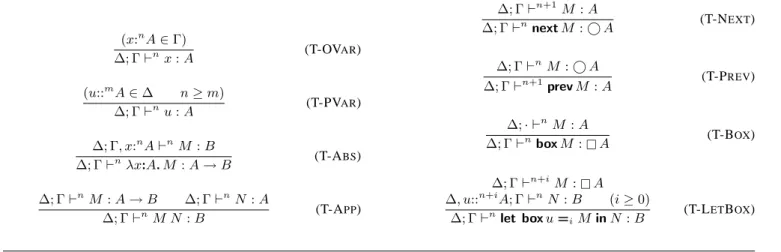
The typing rules to derive type judgments are shown in Fig- ure 1. Each rule is obtained by augmenting each inference rule in the previous section with term constructors. The rules T-OV

AR

and T-PV

AR

correspond to the proof rules for truth and valid assump- tions, respectively. Notice that a declaration u::

ⁿ

A in a persistent context can be referred to at any time equal to or later than n. The rules T-OV

AR

, T-A

BS

, and T-A

PP

for variables, abstractions, and applications, respectively, are essentially the same as ones in the simply typed λ calculus. Notice that the times of type judgments in the premises and conclusions must be the same.

An intuitive meaning of the other rules, related to code types

° A and ¤ A, are explained in the previous section. As already mentioned, T-L

ET

B

OX

allows to unquote persistent code M of time n + i (i ≥ 0), which can be later than the time of the body N. Allowing i > 0 seems necessary to “prove” both ° ¤ A →

¤ ° A and ¤ ° A → ° ¤ A for any A. The next example shows such usage of T-L

ET

B

OX

.

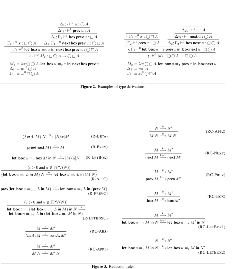
E

XAMPLE

1 (¤ ° A ↔ ° ¤ A).

Let M

1

≡ λx: ¤ ° A. let box u =

0

x in next box prev u and

M

2

≡ λx:° ¤ A. let box u =

1

prev x in box next u. Then, we

(x:

ⁿ

A ∈ Γ)

∆; Γ `

ⁿ

x : A (T-OV

AR

)

(u::

^m

A ∈ ∆ n ≥ m)

∆; Γ `

ⁿ

u : A (T-PV

AR

)

∆; Γ, x:

ⁿ

A `

ⁿ

M : B

∆; Γ `

ⁿ

λx:A. M : A → B (T-A

BS

)

∆; Γ `

ⁿ

M : A → B ∆; Γ `

ⁿ

N : A

∆; Γ `

ⁿ

M N : B (T-A

PP

)

∆; Γ `

ⁿ⁺¹

M : A

∆; Γ `

ⁿ

next M : ° A (T-N

EXT

)

∆; Γ `

ⁿ

M : ° A

∆; Γ `

ⁿ⁺¹

prev M : A (T-P

REV

)

∆; · `

ⁿ

M : A

∆; Γ `

ⁿ

box M : ¤ A (T-B

OX

)

∆; Γ `

ⁿ⁺ⁱ

M : ¤ A

∆, u::

ⁿ⁺ⁱ

A; Γ `

ⁿ

N : B (i ≥ 0)

∆; Γ `

ⁿ

let box u =

i

M in N : B (T-L

ET

B

OX

)

Figure 1. Typing rules

have typing derivations ·; · `

⁰

M

1

: ¤ ° A → ° ¤ A and

·; · `

⁰

M

2

: ° ¤ A → ¤ ° A as shown in Figure 2. Note that in the latter case the T-L

ET

B

OX

rule allows the box code to be used at a time different from that of the code itself.

Closed terms of these types, together with those of types ¤ A → A and ¤ A → ¤ ¤ A (they are axioms of S4 modal logic) for any A, make it possible to convert any code type F

1

· · · F

n

A, where F

i

stands for either ° or ¤, to a “normalized” code type

° · · · ° ¤ A or ° · · · ° A—which concisely expresses at which time code is available—and back.

3.3 Operational Semantics

We define the operational semantics of λ

^°¤

with the (ternary) reduction relation M −→

^k

M

⁰

, read “term M reduces to M

⁰

in one step k stages later.” The index k can be negative. The reduction rules are shown in Figure 3. We simply write M −→ M

⁰

if M −→

^k

M

⁰

for some k and −→

^∗

for the reflexive and transitive closure of −→.

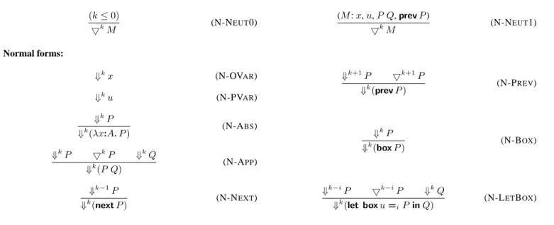
The rule R-B

ETA

is for the standard β-reduction. The R-P

REV

is for unquoting of (ephemeral) code expression. Note that the in- dex is −1 since the redex is typically under another quotation of the previous stage and unquoting happens during the execution of the previous stage. The rule R-L

ET

B

OX

is for embedding persis- tent code expression; if u appears not under box, the quoted code N will run during the execution of the current stage. The rules R-A

PP

C, R-P

REV

C, and L

ET

B

OX

C are for commuting conver- sions, we mentioned in the previous section. We provide congru- ence rules, RC-A

BS

etc., for each term constructors, as we as- sume a full reduction system here. Note that some term construc- tors change the time of the term, so the index k should be changed accordingly.

E

XAMPLE

2. Let M ≡ prev(let box u =

2

box P in Q). Then, M −→

¹

prev([P/u]Q) by R-L

ET

B

OX

, RC-P

REV

and

M −→

⁻¹

let box u =

1

boxP in prev Q by R-P

REV

C.

3.4 Properties of λ

^°¤

The calculus λ

^°¤

enjoys basic properties such as subject reduc- tion, confluence and strong normalization, which are proved in a fairly standard manner.

T

HEOREM

1 (Subject Reduction). If ∆; Γ `

ⁿ

M : A and M −→

M

⁰

, then ∆; Γ `

ⁿ

M

⁰

: A.

T

HEOREM

2 (Confluence). For any term M , if M −→

^∗

M

1

and M −→

^∗

M

2

, then there exists some term N such that M

1

−→

^∗

N and M

2

−→

^∗

N .

T

HEOREM

3 (Strong Normalization). If ∆; Γ `

ⁿ

M : A, then there exists no infinite reduction sequence such that M −→

M

1

−→ · · · −→ M

n

−→ · · ·.

Now, we give a rigorous formalization and proof for time- ordered normalization. The intuitive meaning of time-ordered nor- malization is that, in staged execution of a well-typed program, ear- lier stage execution never requires that of future stages. In other words, having finished its execution at stage n, program execution never goes back to this finished stage. This property is stronger than the property such as “suitably defined call-by-value evaluation can realizes staged computation,” which we will prove in the next sec- tion, because, here, a reduction strategy within a stage is arbitrary (as long as normal forms can be obtained with it).

Time-ordered normalization is first introduced by Davies and proved for λ

^°

[5], which is a subset of λ

^°¤

. His formulation (statement and proof), however, was somewhat informal and even limited to β-reduction: he showed that the time of β-redices can be ordered, assuming R-P

REV

is applied to all redices of the form prev nextM between two β-reductions. In contrast, we state that property in a more formal and general manner, taking all kinds of reduction including R-B

ETA

, R-P

REV

, and R-L

ET

B

OX

and even commuting conversions.

To make a formal statement, we introduce the relation ⇓

ⁿ

M , read “term M is a normal form w.r.t. the times less than n,” together with an auxiliary judgment 5

ⁿ

M, read “term M is neutral w.r.t.

the times less than n,” which are defined by rules in Figure 4. ⇓

ⁿ

M means that there exists no M

⁰

such that M −→

^m

M

⁰

for any m < n, M

⁰

and, 5

ⁿ

M that sustituting M for a variable in any (well-typed) term does not yield a new redex at an earlier time. Note that let box is not neutral, since substituting let box for x in, say, x N yields a new redex due to commuting conversion.

Then, the time-ordered normalization theorem can be stated as below. We write M −→

^k

/ if there exists no M

⁰

such that M −→

^k

M

⁰

.

T

HEOREM

4 (Time-Ordered Normalization). If ∆; Γ `

ⁿ

M : A

and ⇓

^k

M , then for any series of reductions at time k such that

M −→

^k

M

⁰

−→ · · ·

^k

−→

^k

N −→, it holds that

^k

/ ⇓

^k+1

N.

·; Γ

1

`

⁰

x : ¤ ° A

∆

1

; · `

⁰

u : ° A

∆

1

; · `

¹

prev u : A

∆

1

; Γ

1

`

¹

box prev u : ¤ A

∆

1

; Γ

1

`

⁰

next box prev u : ° ¤ A

·; Γ

1

`

⁰

let box u =

0

x in next box prev u : ° ¤ A

·; · `

⁰

M

1

: ¤ ° A → ° ¤ A

M

1

≡ λx: ¤ ° A. let box u =

0

x in next box prev u

∆

1

≡ u::

⁰

° A Γ

1

≡ x:

⁰

¤ ° A

·; Γ

2

`

⁰

x : ° ¤ A

·; Γ

2

`

¹

prev x : ¤ A

∆

2

; · `

¹

u : A

∆

2

; · `

⁰

next u : ° A

∆

2

; Γ

2

`

⁰

box next u : ¤ ° A

·; Γ

2

`

⁰

let box u =

1

prev x in box next u : ¤ ° A

·; · `

⁰

M

2

: ° ¤ A → ¤ ° A

M

2

≡ λx:° ¤ A. let box u =

1

prev x in box next u

∆

2

≡ u::

¹

A Γ

2

≡ x:

⁰

° ¤ A

Figure 2. Examples of type derivations

(λx:A. M) N −→

⁰

[N/x]M (R-B

ETA

) prev(next M ) −→

⁻¹

M (R-P

REV

) let box u =

i

box M in N −→

ⁱ

[M/u]N (R-L

ET

B

OX

)

(i > 0 and u 6∈ FPV(N ))

(let box u =

i

L in M) N −→

⁰

let box u =

i

L in (M N) (R-A

PP

C) prev(let box u =

i+1

L in M ) −→

⁻¹

let box u =

i

L in (prev M ) (R-P

REV

C) (j > 0 and u 6∈ FPV(N ))

let box t =

i

(let box u =

j

L in M ) in N −→

ⁱ

let box u =

i+j

L in (let box t =

i

M in N)

(R-L

ET

B

OX

C) M −→

^k

M

⁰

λx:A. M −→

^k

λx:A. M

⁰

(RC-A

BS

) M −→

^k

M

⁰

M N −→

^k

M

⁰

N (RC-A

PP

1)

N −→

^k

N

⁰

M N −→

^k

M N

⁰

(RC-A

PP

2)

M −→

^k

M

⁰

nextM −→

^k+1

next M

⁰

(RC-N

EXT

)

M −→

^k

M

⁰

prev M −→

^k−1

prev M

⁰

(RC-P

REV

)

M −→

^k

M

⁰

box M −→

^k

box M

⁰

(RC-B

OX

)

M −→

^k

M

⁰

let box u =

i

M in N −→

^k+i

let box u =

i

M

⁰

in N

(RC-L

ET

B

OX

1)

N −→

^k

N

⁰

let box u =

i

M in N −→

^k

let box u =

i

M in N

⁰

(RC-L

ET

B

OX

2)

Figure 3. Reduction rules

Neutral terms:

(k ≤ 0)

5

^k

M (N-N

EUT

0) (M : x, u, P Q, prev P )

5

^k

M (N-N

EUT

1)

Normal forms:

⇓

^k

x (N-OV

AR

)

⇓

^k

u (N-PV

AR

)

⇓

^k

P

⇓

^k

(λx:A. P ) (N-A

BS

)

⇓

^k

P 5

^k

P ⇓

^k

Q

⇓

^k

(P Q) (N-A

PP

)

⇓

^k−1

P

⇓

^k

(next P ) (N-N

EXT

)

⇓

^k+1

P 5

^k+1

P

⇓

^k

(prev P ) (N-P

REV

)

⇓

^k

P

⇓

^k

(box P ) (N-B

OX

)

⇓

^k−i

P 5

^k−i

P ⇓

^k

Q

⇓

^k

(let box u =

i

P in Q) (N-L

ET

B

OX

)

Figure 4. Neutral terms and normal forms

To prove this theorem, we need to show the property that any reduction at time k for M (such that ⇓

^k

M ) does not yield a new redex at an earlier time, or formally:

If ∆; Γ `

ⁿ

M : A and ⇓

^k

M and M −→

^k

M

⁰

, then ⇓

^k

M

⁰

. This property, unfortunately, as it is cannot be proved by induction on M −→

^k

M

⁰

. A problematic case is when M ≡ P Q −→

^k

P

⁰

Q ≡ M

⁰

is derived from P −→

^k

P

⁰

. It must not happen that P

⁰

is a λ-abstraction and k > 0 (otherwise P

⁰

Q −→

⁰

R for some R), but the induction hypothesis would not give such a guarantee.

So we should take neutral terms into account and strengthen the statement to get Theorem 5 below, which we can now prove by straightforward induction on M −→

^k

M

⁰

. Theorem 4 follows from Theorem 5 as a corollary.

T

HEOREM

5 (Reduction Preserves Normality and Neutrality). If

∆; Γ `

ⁿ

M : A and ⇓

^k

M and M −→

^k

M

⁰

, then ⇓

^k

M

⁰

holds and 5

^k

M implies 5

^k

M

⁰

.

Proof. By induction on the derivation of M −→

^k

M

⁰

, with a case analysis of the last rule used. Similarly to subject reduction, we need a lemma that substitution preserves normality and neutrality:

1. If ∆; Γ, x:

^m+i

B `

^m

M : A and ⇓

^k

M and ∆; Γ `

^m+i

N : B and ⇓

^k−i

N and k ≤ i, then, ⇓

^k

([N/x]M ) holds and 5

^k

M implies 5

^k

([N/x]M ).

2. If ∆, u::

^m+i

B; Γ `

^m

M : A and ⇓

^k

M and ∆; · `

^m+i

N : B and ⇓

^k−i

N and k ≤ i, then, ⇓

^k

([N/u]M ) holds and 5

^k

M implies 5

^k

([N/u]M ).

Both (1) and (2) are proved by induction on the structure of M . Now, we show a few representative cases:

Case M ≡ let box u =

i

box P in Q reduces to M

⁰

≡ [P/u]Q by R-L

ET

B

OX

: (Then, k must be equal to i.) By T-L

ET

B

OX

and T-B

OX

, there exists type B s.t. ∆; · `

ⁿ⁺ⁱ

P : B and ∆, u::

ⁿ⁺ⁱ

B; Γ `

ⁿ

Q : A. By ⇓

^k

M and N-L

ET

B

OX

, we have

⇓

^k−i

P , 5

^k−i

P and ⇓

^k

Q. Applying the lemma above, we have

⇓

^k

M

⁰

. If k ≤ 0, it is trivial that 5

^k

M implies 5

^k

M

⁰

; otherwise, it vacuously holds, since M is not neutral, then.

Case M ≡ P Q reduces to M

⁰

≡ P

⁰

Q, with P −→

^k

P

⁰

by a congruence rule: By T-A

PP

, there exists some type B s.t.,

∆; Γ `

ⁿ

P : B → A and ∆; Γ `

ⁿ

Q : B. By ⇓

^k

M and N-A

PP

, we have ⇓

^k

P , 5

^k

P and ⇓

^k

Q. By the induction hypothesis, we have ⇓

^k

P

⁰

and 5

^k

P

⁰

. Therefore by N-A

PP

, we have ⇓

^k

(P

⁰

Q), i.e., ⇓

^k

M

⁰

. Moreover, we have 5

^k

M

⁰

(≡ P

⁰

Q). u t

4. Mini-ML

^°¤

In this section, we extend λ

^°¤

with some basic types, conditional expressions, local definitions, and recursion to obtain Mini-ML

^°¤

, in which examples shown in Section 2.4 are expressible, and give its call-by-value reduction semantics.

4.1 Syntax

We choose our small language to have: (1) Boolean type bool and its literal values true, false, as well as if–then–else construct; (2) integer type int and its literal values . . . , −1, 0, 1, 2, . . ., as well as arithmetic operations of subtraction, multiplication and equality comparison; (3) fix operator for recursive function definitions; and (4) let construct for local definitions. The definition of types and additional terms is shown below.

types A, B ::= bool | int | A → B | ° A | ¤ A terms L, M, N ::= · · · | true | false | if L then M else N

| n | M − N | M ∗ N | M = N

| fix x:A. M | let x = M in N 4.2 Typing Rules

The typing rules for the additional part of our language are quite standard:

∆; Γ `

ⁿ

true : bool (T-T

RUE

)

∆; Γ `

ⁿ

false : bool (T-F

ALSE

)

∆; Γ `

ⁿ

m : int (T-I

NT

)

∆; Γ `

ⁿ

L : bool

∆; Γ `

ⁿ

M : A ∆; Γ `

ⁿ

N : A

∆; Γ `

ⁿ

if L then M else N : A (T-I

F

)

∆; Γ `

ⁿ

M : int ∆; Γ `

ⁿ

N : int

∆; Γ `

ⁿ

M − N : int (T-M

INUS

)

∆; Γ `

ⁿ

M : int ∆; Γ `

ⁿ

N : int

∆; Γ `

ⁿ

M ∗ N : int (T-M

ULT

)

∆; Γ `

ⁿ

M : int ∆; Γ `

ⁿ

N : int

∆; Γ `

ⁿ

M = N : bool (T-E

Q

)

∆; Γ, x:

ⁿ

A `

ⁿ

M : A

∆; Γ `

ⁿ

fix x:A. M : A (T-F

IX

)

∆; Γ `

ⁿ

M : A ∆; Γ, x:

ⁿ

A `

ⁿ

N : B

∆; Γ `

ⁿ

let x = M in N : B (T-L

ET

) 4.3 Call-By-Value Reduction Semantics

Now, we define the call-by-value reduction semantics of Mini- ML

^°¤

in a standard manner using evaluation contexts [7]. Here, formalized is program execution at stage 0, but as we will show this definition suffices: if a program is of type ° A, the resulting quoted code, after unquoting, can run as a new program at stage 0.

First we define the notion of values, taking the meaning of code expressions into account, and then proceed to the definition of the evaluation contexts and call-by-value reduction relation.

4.3.1 Values

The definition of values V

⁽⁰⁾

is given by the following grammar:

D

EFINITION

2 (Values).

V

⁽⁰⁾

, W

⁽⁰⁾

::= true | false | n | λx:A. P | next V

⁽¹⁾

| box P

| let box u =

n+1

V

⁽ⁿ⁺¹⁾

in W

⁽⁰⁾

V

^(k)

, W

^(k)

(k ≥ 1)

::= true | false | n | x | u | λx:A. V

^(k)

| V

^(k)

W

^(k)

| if U

^(k)

then V

^(k)

else W

^(k)

| V

^(k)

− W

^(k)

| V

^(k)

∗ W

^(k)

| V

^(k)

= W

^(k)

| fix x:A. V

^(k)

| let x = V

^(k)

in W

^(k)

| next V

^(k+1)

| prev V

^(k−1)

(k ≥ 2) | box V

^(k)

| let box u =

n

V

^(k+n)

in W

^(k)

Values are constants, function values, or code values (next V

⁽¹⁾

and box P ). Note that V

^(k)

(k ≥ 1), which represents a quoted code fragment at stage k, is not subject to execution at stage 0, thus every term constructor is included. The value of the form let box u =

n+1

V

⁽ⁿ⁺¹⁾

in W

⁽⁰⁾

, which may appear unfamiliar, can be seen as a code value with an environment which binds u to an expression V

⁽ⁿ⁺¹⁾

, whose execution is delayed until stage n + 1. Also note that V

⁽¹⁾

does not include prev V

⁽⁰⁾

; otherwise prev next W

⁽¹⁾

, which should be reduced at stage 0 (cf. R-P

REV

), would be a value.

4.3.2 Evaluation Contexts

An evaluation context is a pseudo term that has a hole [·], which indicates the place where the reduction should be happen. In Mini- ML

^°¤

, the hole can be at not only stage 0 as is expected but also

stage 1, due to the possible redex of the form prev next · · · inside next. So, we introduce two kinds of holes—[·], a hole at stage 0, which expects redices for R-B

ETA

, R-L

ET

B

OX

etc. in it, and {·}, a hole at stage 1, which expects those for R-P

REV

etc. in it. Then, left-to-write, call-by-value evaluation contexts E

⁽ⁿ⁾

at stage n are defined as follows:

D

EFINITION

3 (Evaluation Contexts). Evaluation contexts E

⁽ⁿ⁾

are defined as follows, where op stands for −, ∗, or =:

E

⁽⁰⁾

::= [·] | E

⁽⁰⁾

P | V

⁽⁰⁾

E

⁽⁰⁾

| next E

⁽¹⁾

| let box u =

n

E

⁽ⁿ⁾

in P

| let box u =

n+1

V

⁽ⁿ⁺¹⁾

in E

⁽⁰⁾

| E

⁽⁰⁾

op P | V

⁽⁰⁾

op E

⁽⁰⁾

| if E

⁽⁰⁾

then P else Q | let x = E

⁽⁰⁾

in P E

^(k)

(k ≥ 1)

::= {·} (k = 1) | λx:A. E

^(k)

| E

^(k)

P | V

^(k)

E

^(k)

| next E

^(k+1)

| prev E

^(k−1)

| box E

^(k)

| let box u =

n

E

^(k+n)

in P

| let box u =

n

V

^(k+n)

in E

^(k)

| E

^(k)

op P | V

^(k)

op E

^(k)

| fix x:A. E

^(k)

| if E

^(k)

then P else Q

| if V

^(k)

then E

^(k)

else Q

| if V

^(k)

then W

^(k)

else E

^(k)

| let E

^(k)

= in P | let V

^(k)

= in E

^(k)

Notice the side condition (k = 1) for {·}.

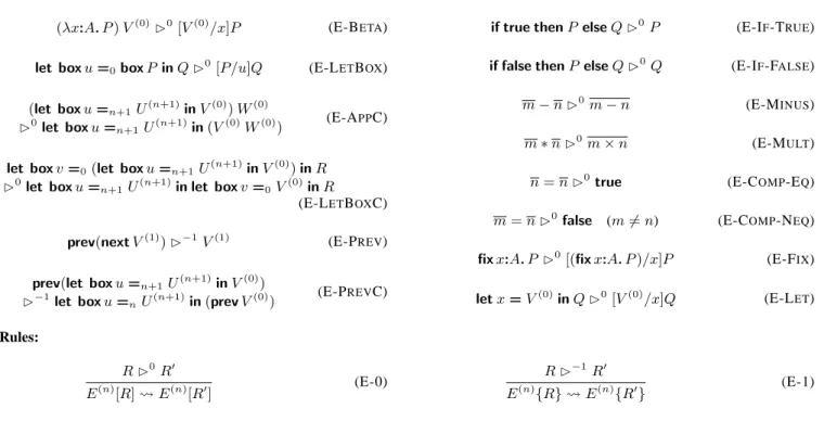
4.3.3 Evaluation Rules

The evaluation rules are shown in Figure 5. P Ã P

⁰

means “term P CBV-reduces to P

⁰

,” while the auxiliary judgment R B

^k

R

⁰

means “redex R reduces to R

⁰

at relative stage k.”

E

XAMPLE

3. We show power cb in Section 2.4 again.

power cb:¤int→ °¤(int→int)

≡λn⁰:¤int. let boxu=n⁰in next boxλx:int. prev(

(fixp:int→°int.λm:int.

ifm= 0then next1

else next(x∗prev(p(m−1)))) u)

The evaluation of power cb (box 2) proceeds in the following way, where p

⁰

is an abbreviation of the part (fix p. . . .) in the definition of power cb, and underlines indicate the place of holes in the evaluation contexts:

power cb(box2)

à let boxu= box2in next boxλx. prev(p⁰u) à next boxλx. prev(p⁰2)

à next boxλx. prev((λm. ifm= 0then next1

else next(x∗prev(p⁰(m−1)))) 2) Ã^∗next boxλx. prev next(x∗prev(p⁰1))

Ã^∗next boxλx. prev next(x∗prev next(x∗prev next1)) Ã next boxλx. prev next(x∗prev next(x∗1))

à next boxλx. prev next(x∗(x∗1)) à next boxλx.x∗(x∗1)

4.4 Properties

The call-by-value reduction defined above is indeed reduction at time 0 in the following sense:

T

HEOREM

6. If ∆; Γ `

⁰

P : A and P Ã P

⁰

then P −→

⁰

P

⁰

.