TRECVID 2008 NOTEBOOK PAPER: Interactive Search Using Multiple Queries and Rough Set Theory

(1)

TRECVID 2008 NOTEBOOK PAPER: Interactive Search Using Multiple Queries and Rough Set Theory

Akihito Mizui

Graduate School of Engineering, Kobe University

1-1, Rokkodai, Nada, Kobe 657-8501, Japan

Kimiaki Shirahama

Graduate School of Economics, Kobe University 2-1, Rokkodai, Nada, Kobe

657-8501, Japan

Kuniaki Uehara

Graduate School of Engineering, Kobe University 1-1, Rokkodai, Nada, Kobe

657-8501, Japan

ABSTRACT

For the TRECVID2008 submitted runs,cs24kobeteam participated in the interactive search task and we submitted two diﬀerent runs:

• 1 b1cs24kobe2 2 : we run the search approach based only on ASR/MT transcripts by using pseudo relevance feedback.

• 1 b2cs24kobe1 1 : we run the search approach based on an exampled-based topic search method which uses multiple queries to “extensionally” deﬁne topics.

Speciﬁcally, we use rough set theory for multiple queries.

There, we can extract subsets of topics, which are characterized by diﬀerent combinations of low-level features. Then, by unifying extracted subsets, we conceptualize the topics.

From the result, even though our result was less eﬀective than expected, we conducted additional experiment to indicate the possibility of our approach. We have learned our approach is eﬀected by user experience on search performances. So, we are currently developing a new approach which can construct the optimal multiple queries by only selecting a few queries.

1. INTRODUCTION

cs24_kobeteam participated in the interactive search task.

Note that since a user can issue a great variety of queries to a large video archive such as TRECVID 2008 dataset, we cannot prepare huge diﬀerent templates for matching shots with these queries. So, we proposed an example-based search approach. This approach ﬁnds shots similar to the query in terms of low-level features. That is, it can directly match shots with queries, and no templates are needed.

However, let us consider the topic of “a red car runs on the street”. Here, low-level features in these topics are changed depending on camera techniques, such as shot sizes and camera angles. For example, a tight shot contains a small amount of motion and a large red region, while a long shot contains a large amount of motion and a small red region.

Like this, a topic consists of subsets which are characterized by significantly different low-level features. Considering this problem, we use multiple examples where each example characterizes a different subset of the topic. That is, we “extensionally” define the topic using multiple examples. We call our example-based approach “query-by-shots”.

To implement our query-by-shots approach, we use rough set theory. In rough set theory, a class is not defined by a single classifier, but is defined by a union of multiple classifiers. By taking advantage of this characteristic, our query-by-shots approach constructs multiple classifiers which separately define subsets of a topic characterized by different combinations of low-level features. By unifying these classifiers, we can collectively search shots belonging to the topic.

In our query-by-shots approach, the selection of examples is very important. For example, classiﬁers learned only from positive examples leads to “over generalization”, because they cannot determine the boundary between positive and negative examples. As a result, a lot of irrelative shots are selected as positive shots. Thus, negative examples are also important for alleviating the over generalization problem. In order to select good positive and negative examples, our query-by-shots approach allows a user to interactively select additional positive and negative examples from a search result (i.e. “query expansion”).

We submitted two diﬀerent runs for the interactive search task:

cs24_kobe1 is the search result byquery-by-shots.

cs24_kobe2 is the search result based only on ASR/MT transcripts. Here, the textual description of a topic is expanded by using pseudo relevance feedback.

In both results, our approach exceeded the time limit because it takes long time to select positive and negative ex-

(2)

amples. Also, some of the results by our query-by-shots approach achieve the average precision, but almost all of results are below the average. The main reason for these bad results is that we only use very simple low-level features, such as color histogram, amount of motion, sound volume and so on.

Nonetheless, we believe that our query-by-shots approach using rough set theory is promising. To show the eﬀec- tiveness of our query-by-shots approach, we conducted an additional experiment. Here, we compared the search result of an experienced user with the one of a naive user.

Clearly, the former result is more accurate than the latter result. But, this experiment indicates an interesting point that a search accuracy depends on a selection of negative examples. Note that the selection of negative examples is a diﬃcult task. As a result, compared to the naive user, the experienced user can select negative examples which are suitable for constructing accurate classiﬁers.

With respect to this point, we are currently developing a new query-by-shots approach which needs no negative examples. Speciﬁcally, we adopt “partially supervised learning”

[6] which can construct a classifier only from positive examples. Here, examples which are completely different positive examples are firstly selected as negative examples. Negative examples are iteratively expanded by clustering currently selected negative examples. Finally, if we can incorporate the partially supervised learning into our query-by-shots approach, we can obtain a robust search result independent of user’s experience.

2. PROBLEMS IN SEARCHING TRECVID VIDEO DATASET

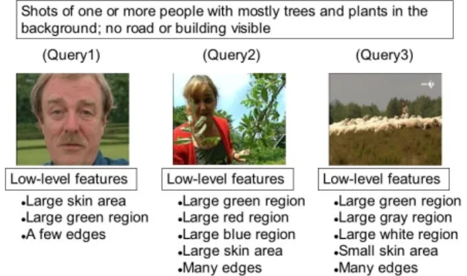
We cannot search semantically meaningful topics by a single query. Let us consider that a user wants to search the 226- th topic “shots of one or more people with mostly trees and plants in the background; no road or building visible”, and provideQuery 2 shown in Fig 1. Fig. 1 represents three examples which are searched by low-level features listed for the 226-th topic. But, a result usingQuery2 only includes shots which show the situations similar toQuery2. It does not include any topics likeQuery1 andQuery3, because it has diﬀerent low-level features fromQuery1 andQuery3.

Like this, in videos, a topic is presented in so many diﬀerent ways, which cannot be captured by a single query. As a result, topic search by a single query is too much speciﬁc and semantically meaningless.

Considering the above problem, we propose a topic search method using multiple queries. It should be noted that we call the existing method “query-by-shot” [1, 13, 16, 14, 7], while we call our method “query-by-shots”. In our query- by-shots method, a user provides multiple queries. Thereby, the user can search shots which show a certain topic, but are presented in diﬀerent shot sizes, such as a tight shot like Query1, a medium shot likeQuery 2 and a long shot like Query 3¹. To implement our query-by-shots method, we

1For a shot, according to the distance between the camera and objects, the shot size is classiﬁed into one of the three types, “tight shot”, “medium shot” or “long shot” [15]. A tight shot is taken by a camera close to objects, while a long

Figure 1: An example of multiple queries.

especially tackle the following problems:

2.1 Inﬁnite number of possible low-level fea- tures

As shown in Fig 1, a topic contains a great variety of low- level features, such as color, edge, motion and audio. So, considering all types of low-level features leads to an inaccurate topic search, where unnecessary low-level features are matched. To overcome this problem, we use data mining technique to extract “patterns” as combinations of statistically correlated low-level features. For example, the 226-th topic is characterized by the pattern “a shot containing large green region and one of more skin area”, because trees and plants have large green region and people have one or more skin area regardless of the size. By using this kind of patterns, we search topics.

2.2 Different subset properties

Shots belonging to a topic are characterized by different combinations of low-level features. In Fig 1, for topics like Query1, “large skin area”, “large green region”, and “a few edges” are important. On the other hand, for topics like Query 3 , “large green region”, “large white region”, “large gray region”, “many edges” and “small skin area” are important. Like this, weights of low-level features are different from each other. Thus, the topic cannot be defined by a single classifier. To overcome this problem, we use rough set theory to extensionally define subsets of shots, and unify them to conceptualize the topic.

2.3 Need for the selection of negative exam- ples

Suppose that we construct a classiﬁer learned only from positive examples, we inevitably search a lot of false positive shots. This result is caused by “over generalization”, because the classiﬁer cannot determine the decision boundary to discern between positive and negative examples. To overcome this problem, we should also select negative examples.

Suppose we search the 226-th topic with a classiﬁer learned shot is taken by a camera distant from objects. A medium shot is taken by a camera, while is placed at an intermediate position between tight and long shots.

(3)

only from positive examples. As shown in Fig. 2 (a), we inevitably search a lot of false positive shots such as the crowd shot. So, we need to select negative examples with similar to these false positive shots as shown Fig. 2 (b)

Figure 2: The negative examples to alleviate the false positive shots for 226-th topic.

However, the selection of negative examples from a huge database is very diﬃcult. For example, in the case of the 226-th topic, we can easily select positive examples such as

“shots have large green region and people”. On the other hand, it is diﬃcult to select negative examples, because the number of examples is too large to select adequate examples to alleviate false positive shots. To overcome this problem, we use interactive search approach, where a user can interactively select additional positive and negative examples from a search result. That is, we have only to select the negative examples from only shots searched as false positive shots. This process is comparatively easy, because the false positive shots are small in number.

Furthermore, we conduct an additional experiment and compare the search results by an experienced user with the ones by a naive user. Then, we indicate the diﬀerence of search performances depending on user experience.

3. QUERY BY SHOTS

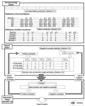
Our query-by-shots method consists of three main phases

“pre-processing”, “search” and “interaction”. In the pre-processing phase, we transform each development and test videos into multistream. Firstly, from each shot, we extract 10 types of low-level features such as color, motion, shift descripior and so on. And, we construct a multistream by sequentially aggregating these low-level features. Secondly we extract patterns as the combinations of statistically correlated low- level features from the set of development videos.

In the search phase, we construct decision rules to find shots relevant to a topic from test videos. Firstly, we select five shots relevant to the topic as positive examples from development videos. Then, negative examples which are irrelevant to the topic are selected from shots without patterns which are contained in positive examples. After that, we use rough set theory for positive and negative examples, and extract a “reduct” which is a minimal set of patterns needed for discerning between positive and negative examples. Based on this reduct, we construct decision rules to find shots rel-

Figure 3: An overview of our query-by-shots method.

evant to the topic from test videos. Finally, we can get a search result.

However, the above search result contains a lot of falsely searched shots. So, we adopt an interaction phase, where we reﬁne decision rules by selecting additional positive and negative examples from the search result. And, we search the topic by using reﬁned decision rules. Finally, we iterate this phase until we get a good search result.

3.1 Low-level Features

A raw video only represents physical values such as RGB values of pixels in each frame. This physical representation is not directly related to semantic contents. Thus, in order to search semantically meaningful topics, we need to derive features which characterize semantic contents. In this work, we deﬁne the following 10 types of low-level features from each shot.

CH, CS, CV: These low-level features respectively represent the color compositions in a keyframe on H(ue), S(aturation) and V(alue) axes of HSV color space. In particular, CH and CS reﬂect the semantic content about the back ground or dominant object, such as plants, sky and so on [2]. On the other hand, CV reﬂects the semantic content of the brightness such as bright and dark. In order to extract the above low- level features, we use the following clustering method.

In the calculation of CH, we ﬁrstly compute the color histogram on H axis for each keyframe. Then, we

(4)

group keyframes into clusters with similar histograms by using k-means clustering algorithm [1]. Here, we use histogram intersection as a distance measure [8].

Finally, for each keyframe, we determine categorical values of CH as the index of the cluster. We can similarly calculate CS and CV by using the abovek-means clustering method.

LN, LL: These low-level features respectively represent the number of edges in a keyframe and the distribution of edge lengths. For example, LN reﬂects the number of objects in the keyframe, that is, the more objects are displayed, the more edges tend to be derived from their boundaries. On the other hand, LL reﬂects objects in the keyframe, that is, buildings and windows have long straight edges, while many short edges are derived from a natural scene [2]. For the extraction of LN, we compare the number of edges with some threshold.

For the extraction of LL, we use the above k-means clustering method.

SA: This low-level feature represents the area of the largest skin colored region in a keyframe. SA reﬂects the size of the main character. Clearly, a large, middle and small skin colored regions are extracted from keyframes where a character appears in a tight, medium and long shot sizes, respectively. For the extraction of SA, we compare the area of the largest skin colored region with some threshold.

SF: This low-level feature represents the histograms, where each bin represents the number of occurrences of particular image patterns. SF reﬂects the local features of objects in the keyframe. For the calculation of SF, we use the following clustering method. Firstly, we construct visual words [9] by clustering the SIFT descriptors using thek-means clustering algorithm. Secondly, we compute SIFT descriptors in each keyframe. And based on the visual words, we construct the histograms of the number of occurrences by quantizing the SIFT descriptors. Finally, we determine categorical values of SF as the index of the cluster by using thek-means clustering algorithm.

AM: AM represents the largest sound volumes in each shot.

For example, a large sound volume reﬂects noisy contents such as military combat, while a small sound volume reﬂects silent contents such as scenery. For the extraction of AM, we extract sound data from each shot and compare them with some threshold.

MV: MV represents the amount of motions in each shot.

MV reﬂects the movements of both objects and the camera. For the extraction of MV, we compare the amount of motion with some threshold.

SL: SL represents the duration of each shot. Generally, in order to emphasize the mood, thrilling events such as battles and chases are presented by shots with short durations, while interviews are presented by shots with long durations. For extracting the low-level feature of SL, we compare the duration of each shot with some threshold.

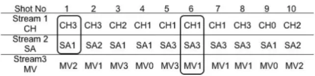
Finally, we sequentially aggregate the above 10 types of low- level features. Thereby, development and test videos are represented as 10-dimensional multistreams. For the space lim- itation, we show a 3-dimensinal multistream in Fig. 4. Here, Stream1 represents the color distribution of the keyframe, Stream2 represents the skin area of the keyframe,Stream3 represents the amount of motion in the shot. As can be seen from this multistream, each low-level feature is a symbol which consists of two capital letters representing the type of this low-level feature and the digit representing the categorical value. For example, shot 1 has the symbol CH3, where CH represents the type of color distribution and its categorical value is 3.

Figure 4: An 3-dimensional multistream.

3.2 Pattern Extraction

Since topic search with all types of low-level features lead to an inaccurate topic, we need to the extract combinations of statistically correlated low-level features as pattens. Each patternpl consisting oflsymbols can be formulated as follows:

pl=V1V2V3 · · · Vl, (1) Here,Vlrepresents a symbol in multistream. plmeans that l symbols V1,· · ·, Vl are statistically correlated because it often occurs wherelsymbols are simultaneously present (or absent) in a shot. For example, as shown in Fig. 4, we depict the patterns p2 as CH3SA1 and the patternp3 as CH1SA3M V1. Note that the above pattern deﬁnition can only consider patterns consisting of symbols in one shot.

Ideally, we should also consider patterns consisting of symbols in consecutive shots by borrowing the pattern deﬁnition introduced in [10]. This is currently a future work.

In order to eﬃciently extract patterns from multistreams of development videos, we use Apriori algorithm which is the most famous algorithm for reducing a search space of possible patterns [12]. This algorithm is outlined as follows:

step 1: We start from l = 1. Then, extract all p1 which satisﬁes a measure of “support”. Here, the support is the frequency ofpland represents its statistical signif- icance.

step 2: Incrementl, and use Apriori algorithm to generate a set of candidate patternscplfrom the set of patterns pl−1 extracted in the previous iteration.

step 3: Count the number ofcploccurrences in the multistream. Then, we measure the usefulness ofcplby using its support and “conﬁdence”. Here, the conﬁdence ofcpl is the conditional probability of one symbol in pl given the other l−1 symbols. This represents a dependence among symbols in cpl. Afterwards, only

(5)

ifcplexceeds both the minimum threshold of support and the one of conﬁdence, we regardcplaspl. step 4: If noplis extracted, terminates the above process.

Otherwise, go to step 2.

In this way, we can eﬃciently extract the patterns of statistically correlated low-level features, by removing unnecessary low-level features from all types low-level features.

3.3 Negative Example Selection

To determine the optimal decision boundary, we need to select negative examples which have completely diﬀerent semantic content from positive examples.

In Fig. 5, we explain the concept of our negative example selection method based on the “temporal locality” [10]. The temporal locality means that topic semantic contents are sequentially presented shot by shot, it is likely that if the same pattern occurs in temporally close shots, they proba- bly show the same semantic content. Based on this temporal locality, we make the following two assumptions. The ﬁrst one is that a semantic content related to positive examples should be continuously presented in an interval. In this interval, the patterns contained in positive examples occur in temporally close shots. In contrast, the second assumption is that a semantic content irrelevant to positive examples is presented in an interval. In this interval, the patterns in positive examples occur in temporally distant shots(or they do not occur in any positive examples). So, we select negative examples from such intervals.

Figure 5: Concept our negative example selection.

For the sake of simplicity, suppose that only the following two patterns are contained in positive examples. As can be seen from Fig. 5, M A2 frequently occurs in the interval from 6-th to 14-th shot, and SM2CH4 frequently occurs in the interval from 5-th to 14-th shot. We select negative examples from intervals, whereSA0M A2 andSM2CH4 do not occur, that is, we select negative examples from 1-th to 4-th shot and the one from 15-th to 18-th shot.

We implement the above negative example selection method in a simple manner. Firstly, we detect intervals where a pattern occurs in temporally close shots based on the following criterion: these intervals have to include more than 4 occurrences of the pattern, and each gap between one occurrence and the previous one has to be less than 2 shots. For each pattern, we use the above criterion to detect intervals where the pattern occurs in temporally close shots. As a result,

we can ﬁnd intervals where the patterns do not occur in any positive examples satisﬁes the above criterion. This means that all patterns in positive examples occur in temporally distant shots, or they do not occur in any shots. From these intervals, we randomly select shots as negative examples.

Ideally, we should use a probabilistic method to robustly detect intervals where a pattern occurs in temporally close shots. A promising method for this purpose is proposed in [8].

3.4 Rough Set Theory

Generally, rough set theory is useful for defining a class which consists of subsets characterized by different attribute values. So, this class cannot be defined by a single classifier. In order to define such a class, rough set theory uses multiple classifiers, each of which characterizes one subset of the class. And, it unifies these classifiers to define the class. In our case, a topic contains multiple subsets which are characterized by different combinations of low-level features. So, we use rough set theory to extensionally define the subsets of a topic, and unify them to conceptualize the semantic content of the topics.

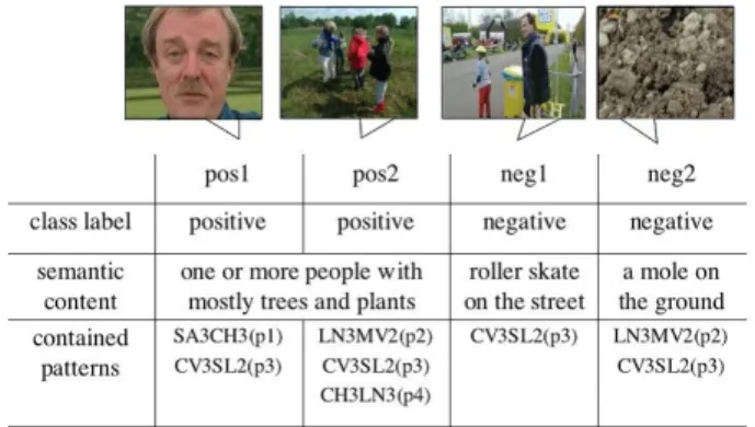
In Fig. 6, we explain rough set theory for a topic search.

pos1 and pos2 represent positive examples, and they have the same semantic content, that is, “one or more people with mostly trees and plants”, which is the 226-th topic. On the other hand,neg1 andneg2represent negative examples, and they have diﬀerent semantic contents, that is, “roller skate on the street” and “a mole on the ground”, respectively.

And these four examples contain four patterns p1, p2, p3

and p4. The pattern p1 is SA3CH3 and it represents “a large green colored region and a large skin codored region”, the pattern p2 is LN3M V2 and it represents “many edges and a small amount of motion”, the patternp3 isCV3SL2 and it represents “high brightness of color and middle shot duration”.

Figure 6: Two positive examples pos1 and pos2 and two negative examples neg1 and neg2 for the 226-th topic.

Then, we represent the above examples in the form of decision table, as shown in Table 1. Here, patterns are used to decide the class label of each example (i.e. positive or negative). Thus, from the decision table, rough set theory

(6)

extracts a minimal set of patterns, which are needed to discern between positive and negative examples. This minimal set is called a “reduct”.

In order to extract a reduct from Table 1, we need to construct the “discernibility matrix”². This matrix represents the diﬀerence between two examples, and are represented as n×nsymmetric matrix. Here,nis the number of examples in Table 1.

Table 1: The decision table for pos1, pos2, neg1 and neg2

.

p1 p2 p3 p4 class label

pos1 1 0 1 0 positive

pos2 0 1 1 1 positive

neg1 0 0 1 0 negative

neg2 0 1 1 0 negative

In Table 2, we explain how to construct this matrix from the decision table. If two examples have the same class label, we fill the corresponding cell withφ, because we do not need to discern the examples. On the other hand, if two examples have different class labels, we fill the corresponding cell with patterns which are contained only in one of the examples.

For example, in Table 1, we can see that pos1 and neg1

have different patternp1, so we fill the corresponding cell withp1 in Table 2. Similarly,pos2 and neg1 have different patternsp2 andp4, so we fill the corresponding cell withp2

and p4. That is, this table indicates that we can discern pos1fromneg1in terms ofp1, similarly we can discernpos2

fromneg1 in terms ofp2 and p4. That is, we can classify one positive example and one negative example by patterns at one corresponding cell.

Table 2: The discernibility matrix forpos1,pos2,neg1

andneg2

.

pos1 pos2 neg1 neg2

pos1 φ

pos2 φ φ

neg1 p1 p2, p4 φ neg2 p1, p2 p4 φ φ

However, we need the classiﬁer to classify all positive examples and negative examples in Fig. 6. So, we use “discernibility f unction fA”. Adiscernibility f unction fAfor an information table A is a Boolean function ofm Boolean variables p^∗₁,. . . ,p^∗_m (each one corresponds to the one of attributes p1,. . .,pm respectively) and is deﬁned as follows:

fA(p^∗1, . . . , p^∗m) =^ {_

c^∗ij|1≤j≤i≤n, cij̸=∅} (2) wherec^∗_ij={p^∗|p∈cij},mis the number of patterns, and nis the number of examples. Speciﬁcally, from Table 2, we

2Here, LetA be an information table with n shots. The discernibility matrix of A is a symmetric n × n matrix with entriescij as given below.

cij={p∈A|p(xi)̸=p(xj)f or i, j= 1, . . . n}

Each entry thus consists of the set of attributes upon which examplesxiandxj diﬀer.

can derive the following discernibility function:

fA(p1, p2, p3, p4) = p1∧(p1∨p2)∧(p2∨p4)∧p4 (3)

= p1∧p4 (4)

By simplifying equation (3), we obtain equation (4). This indicates the reduct is consisting ofp1 andp4. This means that we can classify positive and negative examples by sim- ply usingp1and p4 in Fig. 6.

Based on this reduct, we can construct the “minimal decision rules”. Each of them is constructed as an if-then rule which is constructed by the smallest number of patterns to determine the class label of an example. Speciﬁcally, from the reduct p1∧p4, we can construct following minimal decision rules:

IF(p1) = 1∧(p4) = 0, T HEN class label=positive (5) IF(p1) = 0∧(p4) = 1, T HEN class label=positive (6) IF(p1) = 0∧(p4) = 0, T HEN class label=negative (7)

In particular, the equation (5) represents that we needp1 to obtain the 226-th topic taken by tight shots likepos1, while we don not need p4. Reversely, the equation (6) represents that we needp4 to obtain the 226-th topic taken by a shot with many edges like pos2, while we do not need p1. In this way, by using rough set theory we can define subsets of the 226-th topic which are characterized by different combi- nation of patterns. And by unifying these subsets, we can define semantically meaningful 226-th topic.

Next, we explain how to classify an unseen example from test collections. Below, for the sake of simplicity, we call a minimal decision rule of positive examples and that of negative examples as “positive decision rules” and “negative decision rules”, respectively. We classify an unseen examples into positive, only if the number of positive vote is lager than a threshold and the number of negative vote is less than another threshold. Here, the positive vote is a total number of training data which satisﬁes the positive decision rules, similarly, the negative vote is a total number of training data which satisﬁes the negative decision rules. Finally, such positive examples are output as the result of a topic search.

3.5 Interactive Search

In actual cases, in one trial we cannot classify almost of all shots well. One of the important factors is that it is difficult to select negative examples, because database is too large to select adequate negative examples. To overcome this problem, we interactively add negative examples to existing queries. By iterating search, the selection of negative examples becomes comparatively easy. That is, a user has only to select the negative examples from only shots searched as false positive shots. This process is easy, because the false positive shots are small in number. As shown in Fig. 8, we represent the change of decision boundary by adding negative examples. Here,NandN^′represent existing and added negative examples, respectively. In Fig. 8 (a), a lot of negative shots are wrongly classified as positive shots, because negative examples N are too small. So, we add negative examples N^′ to N and we redefine decision boundary. As shown in Fig. 8 (b), by iterating this process, we get suitable

(7)

Query by Shots (cs24_kobe1)

Text-based (cs24_kobe2)

Figure 7: Summary of our query-by-shots and text-based methods.

decision boundary. That is, we can alleviate a lot of false positive shots, and the precision of classiﬁer is improved.

However, if we only iterate adding negative examples, we cannot correctly deﬁne the decision boundary as shown in Fig. 9 (a). So, we also should add positive examples to existing queries. That is, by adding positive examples, we redeﬁne the decision boundary correctly. As shown in Fig.

9, we represent the change of decision boundary by adding positive examples. Here, P and P^′ represent existing and added positive examples, respectively. In Fig. 9 (a), a lot of positive shots are wrongly classiﬁed as negative shots, because positive examplesP are too small. So, we add positive examplesP^′ to P and we redeﬁne decision boundary.

As shown in Fig. 9 (b), by iterating this process, we get suitable decision boundary. That is, we can get a lot of true positive shots, and the recall of classiﬁer is improved. In this way, in order to deﬁne the decision boundary we need to add positive and negative examples to existing queries interactively.

Figure 8: By adding negative examples, the preci- sion of the classiﬁer will be improved. (a) Without addingN. (b) AddingN^′ to N.

4. EXPERIMENTAL RESULTS

In this section, we describe the search performances of our query-by-shots and text-based methods. In particular, we

Figure 9: By adding positive examples, the recall of the classiﬁer is improved. (a) Without adding P.

(b) Adding P^′ toP.

conduct an additional experiment about our query-by-shots method in order to investigate the eﬀects of user experience on search performances.

4.1 Summary of Submitted Search Results

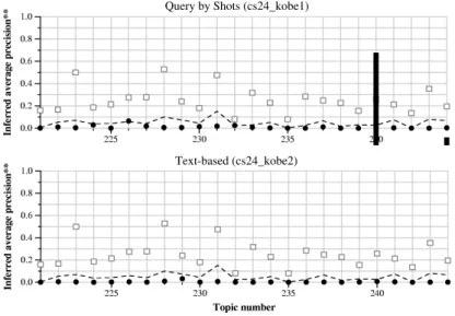
Fig. 7 shows the summary of submitted search results by our query-by-shots and text-based methods. In Fig. 7, for each topic arranged on the horizontal axis, a dot represents the infAP (inferred average precisions) of our search method, while a rectangle represents the infAP of the best search method. Also, the dashed line represents medians of infAPs of all search methods.

For our query-by-shots method, infAPs of some topics such as 224-th and the 226-th are similar to medians, but infAPs of most topics are lower than medians. The main reason for these bad search performances is that our current query- by-shots method only uses simple low-level features, such as color histogram, number of edges, amount of motion, sound volume and so on. As a result, our query-by-shots method cannot precisely discriminate shots relevant to a topic from shots irrelevant to this topic. For example, the search result

(8)

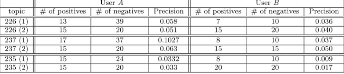
Table 3: Comparison of search results by the userA with the ones by the userC

UserA UserB

topic # of positives # of negatives Precision # of positives # of negatives Precision

226 (1) 13 39 0.058 7 10 0.036

226 (2) 15 20 0.051 15 20 0.040

237 (1) 17 37 0.1027 8 10 0.037

237 (2) 15 20 0.063 15 15 0.050

235 (1) 15 24 0.0332 8 10 0.009

235 (2) 15 20 0.033 20 20 0.017

of 221-th topic “shots of a person opening a door” mainly includes shots containing “long straight lines” and “relatively large amounts of motion”. But, these low-level features are contained in many shots irrelevant to 221-th shots, such as shots in the bottom row in Fig. 10. But, as can be seen from the top row in Fig. 10, our query-by-shots method can search shots which are relevant to 221-th topic but are taken by diﬀerent shot sizes. Thus, if our query-by-shots method uses detailed image and video features such as color layout and edge histogram [3] and keypoint movements, we believe that current search results can be signiﬁcantly improved.

TP-1 (close-up):

130-th shot in BG_38157 TP-2 (tight shot):

39-th shot in BG_36695 TP-3 (medium shot):

133-th shot in BG_38696 TP-4 (long shot):

137-th shot in BG_36618

FP-1:

53-th shot in BG_34992 FP-2:

1-th shot in BG_38011 True

positive

False positive

FP-1: A character talks and gestures with a background involving long straight lines FP-2 and FP-3: A character walks in a building where objects with long straight lines are located FP-4: CGs with long straight lines move

Figure 10: Examples of shots searched by our query- by-shots method for221-th topic.

4.2 Effects of User Experience on Search Re- sults

We notice that the search result of our query-by-shots method signiﬁcantly change depending on users. Speciﬁcally, in the submitted run by our query-by-shots method, the usersA andCsearched topics from 221-th to 232-th and topics from 233-th to 244-th, respectively (223-th and 225-th topics are searched byB).

Here, the average of infAPs (inferred average precisions) for the topics searched byA is 0.0191, on the other hand, the average infAPs searched by C is 0.0023. This result indicates the average of infAPs byAis an order of magnitude larger than the average of infAPs byC. In what follows, we investigate why diﬀerent users achieve the diﬀerent search results by using our query-by-shots method.

We conduct an additional experiment where, for the same topics, we compare search results by A with those of C.

Table 3 shows search results by A and C for three topics 226-th, 237-th and 235-th. As shown in the ﬁrst column, for each topic,AandCperform two diﬀerent types of searches.

In the ﬁrst type, Aand Ccan select arbitrary numbers of

positive and negative examples, while in the second type, A andCcan select ﬁxed numbers of positive and negative examples. For each user’s search, numbers of positive and negative examples are shown in the second, third, ﬁfth and sixth columns. Also, in order to compute the precisions in the forth and seventh columns, we manually count shots relevant to a topic.

From table 3, we can see that A always performs better searches than C. Below, for this result, we explain two fac- tors resulting from A’s and C’s characteristics. Firstly, in the ﬁrst type of searches,Aselects much larger numbers of positive and negative examples than C. Here, precisions of Aare much larger than those ofC. And, in the forth type of searches, diﬀerences between the precisions ofAand precisions ofCare reduced. Thus, we can say that the numbers of positive and negative examples are important in our query- by-shots method, where more accurate decision rules can be constructed from a larger number of examples.

Secondly, as can be seen from the second type of searches, even ifAandCselect the same numbers of positive and negative examples, precisions ofAare larger than precisions of C. The reason is thatAtends to select negative examples by considering the relation of low-level features between positive and negative examples, whileCtends to select negative examples whenever they are irrelevant to the topic. For example, in the search of the 226-th topic,Cselects the crowd shots as negative examples. But, both of shots showing trees or plants and the crowd shots have a large number of edges, so this selection of the crowd shots as negative examples causes to reduce the number of shots relevant to the 226-th topic.

Note that the selection of positive examples is relatively easy, because they have only to show one kind of semantic content relevant to a topic. On the other hand, the selection of negative examples is difficult and heavily depends on users, because they show various kinds of semantic contents irrelevant to the topic. And, different users select different negative examples, that is, experienced users such asAcan select better negative examples than naive users such asC.

In the near future, to solve this instability of search performances, we will extend our query-by-shots method by adopt- ing “partially supervised learning”, so that decision rules can be constructed only from positive examples.

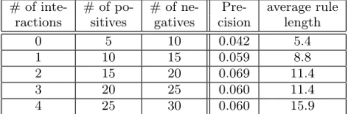
Finally, in order to investigate the above ﬁrst factor more closely, we askAto re-search the 226-th topic and check his search result after each interaction.³ The result is shown in

3For the 226-th topic, the precision at the second interaction

(9)

table 4. Interestingly, in table 4, precisions are gradually improved until the second interaction, while they are degraded from the second to the forth interaction. This can be con- sidered as “over specialization (or overfitting)”. Specifically, complex decision rules constructed from many examples do not necessarily yields an accurate search, as shown in the fifth column which represents average lengths of decision rules. Thus, it is one of our future works to determine the numbers of positive and negative examples which lead to the best search result.

Table 4: Change of precisions by user interactions inA’s search of 226-th topic

# of inte- # of po- # of ne- Pre- average rule ractions sitives gatives cision length

0 5 10 0.042 5.4

1 10 15 0.059 8.8

2 15 20 0.069 11.4

3 20 25 0.060 11.4

4 25 30 0.060 15.9

5. CONCLUSION AND FUTURE WORKS

We have conducted experiments for interactive search tasks in TRECVID-2008. We introduced a query-by-shots topic search method based on the following three key ideas: First, by extending an example-based approach, we use multiple examples to cover the various topics. Second, we use rough set theory and extensionally define the topic. The reason is that a topic cannot be defined by a single example because a topic consists of subsets characterized by different combinations of low-level features. Thus, we define the above subsets and unify them to conceptualize the topic. Third, we adopt an interactive search and interactively expand queries until we get a good search result.

Even though our results were less eﬀective than expected, we believe that our query-by-shots approach using rough set theory is promoting. And so, we list several research issues which should be future explored to improve our approach.

Firstly, we need to improve our some component methods, such as low-level feature extraction method, a pattern extraction method, selection of negative example. In terms of the low-level feature extraction, we need to add the spatial information such as “Spatial pyramid kernel” [11]. Be- cause, some of our low-level features, such as SL are eﬀec- tive in edited video like movie and drama, but they are too low-level to be eﬀective in news video such as TRECVID 2008 dataset. In terms of a pattern extraction, by using our

“Time-costrained Sequential Pattern Mining” [10], we can extract more semantically meaningful patterns with time- constraint. In terms of selection of negative example, we notice that we should select more useful negative examples to ﬁnd suitable decision boundary despite user experience.

Therefore, we adopt “partially supervised learning”, and we aim for robust method to select useful negative examples.

Secondly, we must reduce the search time for the TRECVID 2009. From the additional experiment, we need to improve in table 4 is diﬀerent from the one in the second type of search in table 3. It is becauseA selects diﬀerent positive and negative examples in the above two searches.

our interface to select examples easily. So, we need to adopt a semantic search browser likeCross Browser employed in MediaMill [5].

Finally, we plan to merge our query-by-shots search and the text only search. To achieve it, we need to enhance the precision by text only search, so we are due to adopt the approach based on statistical models for text segmentation [4] to treat colloquial text from news video. And we examine how to merge these approach is more useful.

6. REFERENCES

[1] A. Jain, A. Vailaya and X. Wei. Query by video clip.

Multimedia Systems, 7(5):369–384, 1999.

[2] A. Mojsilovic and B. Rogowitz. Capturing image semantics with low-level descriptors. InProc. of ICIP 2001, pages 18–21, 2001.

[3] B. Manjunath, J. Ohm and V. Vasudevan and A.

Yamada. Color and texture descriptors.IEEE Transactions on Circuits and Systems for Video Technology, 11(6):703–715, 2001.

[4] D. Beeferman, A. Berger and J. Laﬀerty. Statistical models for text segmentaion.Machine Learning, 34:177–210, 1999.

[5] O. de Rooij, C. G. M. Snoek, and M. Worring.

Balancing thread based navigation for targeted video search. InProc. of ACM CIVR 2008, pages 485–494, 2008.

[6] G. Fung, J. Yu, H. Lu and P. Yu. Text classiﬁcation without negative examples revisit.IEEE Transactions on Knowledge and Data Engineering, 18(1):6–20, 2006.

[7] I. Kondo, S. Shimada and M. Morimoto. A video retrieval technique based on the sequence of symbols created by shot clustering (In Japanese).Technical Report of IEICE Multimedia and Virtual

Environment, 106(157):31–36, 2006.

[8] J. Kleinberg. Bursty and hierarchical structures in streams. InProc. of KDD 2002, pages 91–101, 2002.

[9] J. Sivic and A. Zisserman. Video google: A text retrieval approach to object matching in videos. In Proc. of ICCV, pages 1470–1477, 2003.

[10] K. Shirahama, K. Ideno and K. Uehara. A time-constrained sequential pattern mining for extracting semantic events in videos. In V. A.

Petrushin and L. Khan, editors,Multimedia Data Mining and Knowledge Discovery, pages 423–446.

Springer, 2006.

[11] S. Lazebnik, C. Schmid, and J. Ponce. Beyond bags of features: al pyramid matching for recognizing natural scene categories. InProc. of CVPR 2006, pages 2169–2178, 2006.

[12] R. Agrawal and R. Srikant. Fast algorithms for mining association rules. InProc. of VLDB 1994, pages 487–499, 1994.

[13] X. Liu, Y. Zhuang and Y. Pan. A new approach to retrieve video by example video clip. InProc. of ACM MM, pages 41–44, 1999.

[14] Y. Kim and T. Chua. Retrieval of news video using video sequence matching. InProc. of MMM 2005, pages 68–75, 2005.

[15] Y. Matsuo, K. Shirahama and K. Uehara. Video data mining: Extracting cinematic rules from movie. In

(10)

Proc. of MDM/KDD 2003, pages 18–27, 2003.

[16] Y. Peng and C. Ngo. EMD-based video clip retrieval by many-to-many matching. InProc. of CIVR 2005, pages 71–81, 2005.

TRECVID 2008 NOTEBOOK PAPER: Interactive Search Using Multiple Queries and Rough Set Theory