Supervised ordering by regression combined with Thurstone’s model

DOI 10.1007/s10462-007-9050-5

Supervised ordering by regression combined with Thurstone’s model

Toshihiro Kamishima · Shotaro Akaho

Published online: 7 November 2007

© Springer Science+Business Media B.V. 2007

Abstract In this paper, we advocate a learning task that deals with the orders of objects, which we call the Supervised Ordering task. The term order means a sequence of objects sorted according to a specific property, such as preference, size, cost. The aim of this task is to acquire the rule that is used for estimating an appropriate order of a given unordered object set. The rule is acquired from sample orders consisting of objects represented by attri- bute vectors. Developing solution methods for accomplishing this task would be useful, for example, in carrying out a questionnaire survey to predict one’s preferences. We develop a solution method based on a regression technique imposing a Thurstone’s model and evaluate the performance and characteristics of these methods based on the experimental results of tests using both artificial data and real data.

Keywords Order · Rank · Supervised learning · Regression analysis · Thurstone’s law of comparative judgment · Sensory survey

1 Introduction

In this paper, we advocate a new learning task that deals with the orders of objects, which we call Supervised Ordering. Here, the term order means a sequence of objects sorted accord- ing to a specific property. Suppose there are three kinds of meals, x

, x

, and x

. Then one example of order is the sequence x

x

x

, in which the sorting is performed according to Taro’s preference. This order represents that he likes meal x

the most, and meal x

the least. The goal of a supervised ordering task is to acquire the rule that is used for

T. Kamishima (

B

National Institute of Advanced Industrial Science and Technology (AIST), Tsukuba Central 2, Umezono 1–1–1, Tsukuba, Ibaraki, Japan

e-mail: [email protected] URL: http://www.kamishima.net/

S. Akaho

e-mail: [email protected]

estimating an appropriate order for any object set. The rule is learned from training sample orders consisting of objects represented by attribute vectors.

An example of performing a supervised ordering task would be completing a question- naire survey of preferences in meals. The surveyor presents several kinds of meals to each respondent and requests that he/she sort the meals according to his/her preference. By apply- ing a supervised ordering method, the surveyor will be able to estimate the respondents’

preference order of meals, and to determine, for example, the most preferred meal, or the factors affecting preference. For such a survey, it is typical to use the Semantic Differential method (Osgood et al. 1957). By this method, the respondents’ preferences are measured on a scale, the extremes of which are expressed by antonyms:

prefer 5 4 3 2 1 don’t prefer

A proper interpretation of responses using this scale would be, for example, that respon- dents prefer objects categorized as “5” to objects categorized as “4”. However, to analyze the acquired ratings as interval values, that are numerical values the scale and origin of which are free, the following two assumptions must be introduced: “The total lengths of all the scales are equal” and “All the intervals of one scale are equal” (Nakamori 2000). However, it is commonly difficult for respondents to quantify their own sensation so as to satisfy these assumptions. One way to avoid these assumptions is by introducing a ranking method. In this method, the respondents’ sensations or preferences are measured by the orders sorted accord- ing to the target to measure. But this measuring method has not frequently been used due to the lack of an analysis technique. We therefore undertook to develop a learning technique targeting orders.

In this paper, we formally specify the supervised ordering task, then propose its solution method based on a regression technique incorporating Thurstone’s model. We also show Cohen’s method, which was designed for a task close to that of supervised ordering, and its variants. We apply these methods to both artificial and real data, respectively. Analysis of the experimental results revealed the characteristic results of these methods.

We proceed as follows. In Sect. 2, we present the formal specifications of a supervised ordering task. We propose several supervised ordering methods in Sect. 3, and show experi- mental results in Sect. 4. Finally, Sect. 5 summarizes our conclusions.

1.1 Related work

Though research in analysis techniques for orders has not been widely conducted, several previous studies exist. A pioneering work is Thurstone’s law of comparative judgment (Thur- stone 1927). Thurstone proposed a method of constructing a real-value scale from a set of ordered object pairs. The ordinal regression is a regression method adopting models in which dependent variables are ordered categorical type (Agresti 1996; Anderson and Philips 1981;

McCullagh 1980). Some probabilistic models for orders have been developed (Babington

Smith 1950; Fligner and Verducci 1990; Mallows 1957; Plackett 1975). Recently, there has

been active research in the processing of orders. Mannila and Meek (2000) tried to establish

the structure expressed by partial orders among a given set of orders. Sai et al. (2001) proposed

association rules between order variables. Kamishima and Fujiki studied the k-o’means algo-

rithm for clustering incomplete orders (Kamishima and Fujiki 2003). Kamishima developed

collaborative filtering techniques based on order responses (Kamishima 2003). Kamishima

and Akaho proposed a technique for filling-in missing objects in orders (Kamishima and

Akaho 2004). Lebanon and Lafferty discussed the combination method for orders using

conditional probability models (Lebanon and Lafferty 2002).

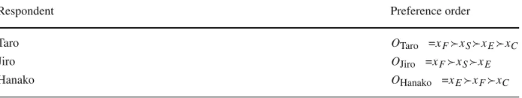
Table 1 Examples of preference orders in sushi

Respondent Preference order

Taro O_Taro =x_Fx_Sx_Ex_C

Jiro O_Jiro =x_Fx_Sx_E

Hanako OHanako =xExFxC

Objects: xC(Cucumber roll), xE(Egg), xF(Fatty tuna), xS(Squid), xT(Tuna)

The task studied by Cohen et al. (1999), Herbrich et al. (1998), and Joachims (2002) is a special case of our task. We later describe these in Sect. 3.1.

2 Supervised ordering

2.1 Basic notations

This section formally states a supervised ordering task.

An object x

corresponds to an object, entity, or substance to be sorted. The universal object set, X

, consists of all possible objects. Each object x

is represented by the attribute value vector, x

= ( x

, x

, . . . , x

) , where k is the number of attributes. In this paper, we focus on the case in which all the attributes are categorical. The l-th attribute can take one of the |v

| values, {v

, . . . , v

}.

The order is denoted by O=x

x

· · · x

. The transitivity is preserved in the same order; i.e., if x

x

and x

x

, then x

x

. To express the order of two objects, x

x

, we use the sentence “x

precedes x

.” X

⊆ X

denotes the object set that is composed of all the objects that appear in the order O

. Let | A | be the size of the set A, then | X

| is equal to the length of the order O

. If X

= X

, an order O

is called a complete order, otherwise it is called an incomplete order. A rank, r(O

, x

), is the cardinal number that indicates the position of the object x

in the order O

.

For two orders, O

and O

, consider an object pair x

and x

, such that x

, x

∈ X

∩ X

, x

= x

. We say that the orders O

and O

are concordant w.r.t. x

and x

, if two objects are placed in the same order, i.e.,

( r ( O

, x

) − r ( O

, x

))( r ( O

, x

) − r ( O

, x

)) ≥ 0 ;

otherwise, these two orders are discordant. O

and O

are concordant if O

and O

are concordant w.r.t. all object pairs such that x

, x

∈X

∩X

, x

=x

.

Table 1 shows three example orders, each of which is sorted according to one respon- dent’s preference in sushi (a Japanese meal). In this case, each object corresponds to a kind of sushi (see note in Table 1), and is represented by the six attributes in Table 8. A universal set is composed of five objects, X

= {x

, x

, x

, x

, x

}. For Taro’s preference order, X

= {x

, x

, x

, x

}, |X

| = 4, and r(O

, x

)=3. O

is incomplete due to the fact X

⊂ X

. Further, O

and O

are concordant w.r.t. x

and x

, but are discordant w.r.t. x

and x

, thus O

and O

are discordant. O

and O

are concordant.

The pair set Pair(O

) is composed of all the object pairs x

x

, such that x

precedes

x

in the order O

. For example, O

is decomposed into three pairs, x

x

, x

x

,

and x

x

. Given a set of orders, S, Pair(S) is composed of all pairs in Pair(O

), O

∈ S.

Note that Pair ( S ) =

Oi∈S

Pair ( O

) , because pairs of the same form are multiply contained in Pair ( S ) . For example, for S = { O

, O

, O

} , Pair ( S ) consists of 12 pairs including two x

x

originated from O

and O

.

2.2 Formalization of a supervised ordering task

The supervised ordering task is composed of two major stages: a learning stage and a sorting stage. In the learning stage, given a set of sample orders, S = {O

, O

, . . . , O

}, the learner acquires a sorting function, sort( X

), that is the function of an unordered object set X

⊆ X

. In the sorting stage, based on the acquired function, sort ( X

) , the constituent objects in X

are sorted in an appropriate order. We denote the estimated order of X

by O ˆ

. For example, suppose that a sorting function is learned from S = { O

, O

, O

} in Table 1.

Given an unordered object set X

= {x

, x

, x

, x

} as an argument of the sorting func- tion, these objects are sorted into an estimated order, say, O ˆ

= x

x

x

x

. This esti- mated order should satisfy the following two conditions: First, the estimated order should be maximally concordant with sample orders in S. The degree of concordance is measured by the similarities between orders as shown later. The above O ˆ

is perfectly concordant with O

or O

, and almost concordant with O

. Second, the objects not appearing in S, e.g., x

in Table 1, have to be sorted by using the sorting function. In an estimated order, the ranks of such unseen objects should be close to those of the objects that are neighbors of the unseen objects in attribute space. For example, the x

(Tuna) is a neighbor of the x

(Fatty Tuna) in an attribute space, thus it would be appropriate that the x

was ranked next to the x

.

We next show a concordance or similarity measure between two orders. In this investi- gation, we adopted the well known statistics Spearman’s Rank Correlation ρ (Kendall and Gibbons 1990), defined as the correlation between ranks of objects. The ρ between two orders, O

and O

, consisting of the same objects (i.e., X

= X

(≡ X ) ) is defined as:

ρ(O

, O

) =

x∈X

r ( O

, x ) − ¯ r

r ( O

, x ) − ¯ r

r(O

, x)−¯ r

x∈X

r(O

, x )−¯ r

, where r denotes the mean rank, i.e., ¯ (1/|X|)

x∈X

r(O

, x). If no tie in rank is allowed, this can be calculated by the simple formula:

ρ(O

, O

) = 1 − 6 ×

x∈X

r(O

, x ) − r(O

, x )

|X|

− |X| .

The ρ becomes 1 if the two orders are perfectly concordant, and −1 if one order is a reverse of the other order. It is known that for two random orders having lengths of |X|, the t-value,

t = ρ

| X | − 2

1 − ρ

, (1)

asymptotically follows the Student t-distribution with degree of freedom |X|−2 (Kendall and Gibbons 1990).

It is worthwhile to point out that this supervised ordering task is connected to the notion of

the center of orders (Marden 1995). A central order is the order to maximize the mean simi-

larity among given sample orders. For finding such central orders, many methods and models

have been developed; for example, Thurstonian type models (Thurstone 1927), a Babington

Smith model (Babington Smith 1950), a Mallows model (Mallows 1957), or a Plackett-Luce

model (Plackett 1975). Unlike those in a supervised ordering task, these sample orders are the sequences of objects that are represented by unique identifiers, not by attribute vectors.

Therefore, methods for finding central orders cannot be used for ordering objects unseen in sample orders. However, the sorting function of a supervised ordering case can be used for sorting unseen objects based on information of their attributes. A supervised ordering task can be considered as an extension of this task so as to deal with objects represented by attribute vectors.

3 Methods

In this section, we describe the two types of solution methods for a supervised ordering task.

One is based on a classification technique and was proposed by Cohen et al. The other is our new method based on a regression technique.

3.1 Cohen classification (CC)

Cohen et al. (1999), Herbrich et al. (1998), and Joachims (2002) studied the task that is the special case of a supervised ordering task. Thus, we first describe this. The main difference in formalization between their task and a supervised ordering task is the length of sample orders. Samples of their task are ordered pairs of objects, i.e., the length of orders are exactly two, whereas any length of samples are allowed in a supervised ordering task. Formally, the learner is given samples of ordered pairs, S

= { P

, . . . , P

} , where P

denotes an order the length of which is two. As in the case of a supervised ordering task, the aim of this task is to acquire the function sort(X

). Note that the size of the unordered object set X

is not limited to two. Objects are again sorted into an order so that they are concordant with given sample pairs, and objects neighboring in attribute space are ranked proximately in the order.

Cohen et al. proposed a sorting function defined by the following procedure. First, the conditional probability function, Pr [ x

x

| x

, x

] , of the event that x

precedes x

given the attribute values of x

and x

is derived from samples. Cohen et al. (1999) used their original Hedge algorithm to learn the probability function. We consider their main contribution to be the sorting procedure using this function, which can be replaced with any algorithm to learn the probability. In addition, their method required adoption of an on-line learning algo- rithm to perform the application task, whereas our application problem can be solved by using off-line algorithms. We therefore adopted a basic and well studied algorithm, the naive Bayes classifier (Mitchell 1997).

Pr[x

x

|x

, x

] ∝ Pr[x

, x

|x

x

] Pr[x

x

], Pr [ x

, x

| x

x

] ≈

Pr [ x

, x

| x

x

].

As the probability Pr[x

, x

|x

x

], we adopt the following Bayesian estimator with the Dirichlet prior so that the probability is non-zero:

Pr [ x

, x

| x

x

] = | x

x

| + |v

|

| S

| + 1 ,

Table 2 Cohen’s Greedy-order Algorithm INPUT: Xu

1) Oˆu← ∅

2) foreach x∈Xudo score(x)←

x∈XuPr[xx|x,x] 3) xtop←arg max_x∈Xuscore(x)

4) Oˆu← ˆOuxtop, Xu←Xu− {xtop},

5) foreach x∈Xudo score(x)←score(x)−Pr[xxtop|x,xtop] 6) if Xu= ∅then goto step 3

7) outputOˆu

where | x

x

| is the total number of the object pairs x

x

such that x

= x

and x

= x

are members of the S

. Pr[x

x

] can be calculated by

Pr[x

x

] = |x

x

| + 0.5

|x

x

| + |x

x

| + 1 , where |x

x

| is the number of the object pairs, x

x

, in the S

.

After having learned such a probability function, an estimated order, O ˆ

, is derived so as to maximize the agreement:

xax_b∈

Pair

Pr [ x

x

| x

, x

], (2)

where Pair( O ˆ

) is a pair set of O ˆ

in Sect. 2.1. To derive O ˆ

, the permutation of X

that maximizes Eq. 2 is searched for among all possible permutations. However, because finding the optimal order is not tractable if | X

| is large, the greedy algorithm in Table 2 is used.

Simply speaking, this algorithm sequentially chooses the most-preceding object according to the function score(x).

To apply Cohen’s method for solving a supervised ordering task, we convert the given sample orders into the form of ordered pairs. Specifically, a sample set of a supervised order- ing task, S, is converted into the pair set, Pair ( S ) , in Sect. 2.1, and the Pair ( S ) is considered as sample pairs of Cohen’s task, S

. From the converted set of ordered pairs, the proba- bility function Pr [ x

x

| x

, x

] can be derived. By applying the above Cohen’s procedure, objects in any unordered set X

will be sorted appropriately. We refer to this method as Cohen Classification (CC).

It is worthwhile to discuss the difference between Cohen’s task and a supervised ordering

task. These two tasks are distinct in terms of the length of sample orders; it must be two in a

Cohen’s, whereas a longer length is allowed in a supervised ordering task. This distinction

seems slight, but affects the following two features: concordance among orders and distri-

butional properties of samples. We first discuss what is an order maximally concordant with

sample orders. Due to the statistical generation nature of sample orders, these orders may

conflict with each other. For example, how should three orders, x

x

, x

x

, and x

x

,

be combined? To resolve such conflicts, preferential conditions must be introduced to induce

combined orders. Such conditions have been studied since the 18th century. For example,

in the literature of social choice, de Condorcet pointed out that there are disagreements

among orders derived by ordering schemes grounded in plausible different policies

(de Condorcet 1995). Arrow proved the Arrow’s impossibility theorem (Arrow 1963); there

is no method to combine orders so as to simultaneously satisfy four plausible conditions called U, P, I, and ND. Among such conditions, we here focus on Arrow’s Condition I:

independence from irrelevant alternatives. Specifically, if a sorting function is fixed, either x

x

or x

x

is concordant with O ˆ

for any X

such that x

, x

∈ X

. In other words, the order with respect to two objects is determined depending on only these two objects. For example, once a sorting function outputted x

x

x

, the function must sort {x

, x

, x

} into orders that are concordant with x

x

, i.e., x

x

x

, x

x

x

, or x

x

x

. In the statistical case, this can be formulated by

Pr[r( O ˆ

, x

) > r( O ˆ

, x

)|X

] = Pr[r( O ˆ

, x

) > r( O ˆ

, x

)|{x

, x

}].

If the lengths of sample orders are two, i.e., Cohen’s case, a sorting function learned from these samples is implicitly assumed to output orders that satisfy this condition because there is no information about the dependency of determination of the order between two objects on the other objects, due to the fact that third objects are not given in sample orders. In a supervised ordering case, in which there are sample orders composed of more than two objects, such information will be available. Therefore, learner cannot learn sorting functions not satisfying Arrow’s Condition I, even if needed. Note that the supervised ordering meth- ods in this paper assume this condition, based on the fact that the condition is preferable in many applications. For example, in the case of the sushi preference survey in Table 1, Fatty Tuna would be preferred to Cucumber Roll, even if any other types of sushi were considered together with these types of sushi.

Moreover, the difference in the length of orders, especially between the orders of the length two and the orders the length of which are longer than two, affects the dependence of objects in sample orders. If sample orders are given in a form of ordered pairs as in Cohen’s case, the independence among pairs would be high. On the other hand, pairs in Pair ( S ) are not highly independent, because if x

x

and x

x

are in Pair(S), there is a high probability that x

x

originated from the decomposition of x

x

x

would also be in Pair(S). There- fore, between task formulations of Cohen’s and of a supervised ordering, the distribution of ordered pairs differs considerably.

3.2 Babington Smith classification (BSC)

As noted in Sect. 2.2, a supervised ordering method can be considered as an extension of a method for finding central orders. That is to say, supervised ordering methods consist of two components: one is an attribute component for mapping attributes to internal representation, the other an ordering component for sorting objects based on the representation. As an attri- bute component of CC, traditional classification modeling is used. However, a model for its ordering part is not found in any traditional models, so its properties are unknown. Hence, we analyzed the properties of CC based on the behavior of its variant method employing an existing ordering model that is very close to that of CC. Below, we show this variant method, which is introduced only for the purpose of analyzing the properties of CC.

By replacing the summation in the Cohen’s criterion (2) with the production, we obtain

x_ax_b∈

Pair

Pr [ x

x

| x

, x

]. (3)

This coincides with the Babington Smith Model (Babington Smith 1950; Marden 1995), that is, the simple and early developed probability model for orders, up to the normalization term.

This model represents the probability of orders under the independence assumption among

ordered pairs. For example, the order x

x

x

is observed under the assumption that the events x

x

, x

x

, and x

x

are independent.

This algorithm is the same as the algorithm in Table 2, except in terms of the calculation steps of scores:

2) foreach x ∈ X

do score ( x ) ←

Pr [ x x

| x , x

] 5) foreach x ∈ X

do score ( x ) ← score ( x )/ Pr [ x x

| x , x

]

We refer to this method as Babington Smith Classification (BSC). The mathematical formulation of BSC is not only similar to that of CC, but also the experimental results in Sect. 4 will show that these methods lead to similar estimated orders.

3.3 Thurstone regression (TR)

In this section, we advocate an alternative solution method based on the regression technique combined with Thurstone’s model. We call this method the Thurstone Regression (TR). We describe this new method, then show why it allows appropriate orders to be estimated.

In the sorting stage of TR, a linear score function of attribute value vector, x

, is used. The score r ˆ ( x

) = w · x

is the inner product of the weight vector w and the x

. The estimated order is derived by sorting the objects x

∈ X

according to the score r ˆ ( x

) . This function is acquired in the learning stage. The learning procedure is composed of two stages. First, the given sample orders are combined into one order based on Thurstone’s model. Second, applying a regression technique derives a linear function r(x ˆ

) to estimate the ranks in this combined order.

We show a derivation process of the combined order. All the object sets in the training example set are collected into one object set, X

, i.e.,

Xi∈S

X

. Next, a central order, that is an order consisting of X

and being maximally concordant with sample orders, is found.

To derive this central order, O

, one creates the set of object pairs Pair(S) and calculates the probabilities for every pair in Pair ( S ) :

Pr[x

x

] = |x

x

| + 0.5

| x

x

| + | x

x

| + 1 ,

where |x

x

| is the number of the object pairs, x

x

, in the Pair( S). These probabilities are applied to Thurstone’s law of comparative judgment (Thurstone 1927); that is, to the generative model of orders. This model assumes that the score is assigned to each object x

. The orders are derived by sorting according to the scores. Scores follow normal distribution;

i.e., N (µ

, σ ) , where µ

is the mean score of the object x

, and σ is a common constant standard deviation. By applying the least square method to this model (Mosteller 1951), the µ

, that is the linear transformation of the µ

, is derived as

µ

= 1

| X

|

x∈Xu

Pr [ x

x ]

, (4)

where (·) is the normal cumulative distribution function. The µ

is derived for each object in X

, and the combined central order O

can be derived by sorting according to these µ

.

After the calculation of the order O

, we then acquire the score function, r ˆ ( x

) , that

measures the degree to which the object x

precedes the other objects. The function r(x ˆ

)

is derived by the regression technique for categorical attributes using dummy variables; this

is also known as the Type 1 Quantification method (Hayashi 1952). First, the attribute value

vector of each object, x

∈ X

, is transformed into the vector d (x

). The first step of this

transformation is to represent x

by the 0–1 dummy vector. For example, consider the trans- formation of the attribute value vector x

=(v

, v

, v

) , and the 1st, 2nd, and 3rd attribute can take {v

, v

} , {v

, v

, v

} , and {v

, v

} , respectively. This vector is converted into

x

⇒ ( 0 1 v

v

x

1 0 0

v

v

v

x

1 0

v

v

x

).

The d(x

) is then derived by eliminating the 0–1 entries corresponding to the first values except in terms of the first attribute. Namely, the entries v

, v

, . . . , v

are deleted. In the case of the above example, the entries v

and v

are deleted, and we obtain

d ( x

) = ( 0 1 v

v

x

0 0

v

v

x

0 v

x

).

Such d(x

) are derived for each element x

in X

, and the examples, (r(O

, x

), d(x

)), are formed. By applying the standard regression method to this example set,

{(r(O

, x

), d (x

)), (r(O

, x

), d(x

)), . . . , (r( O

, x

), d(x

))},

we obtain the weight vector, w. The dependent and independent variables of this regres- sion model are r(O

, x

) and d(x

), respectively. Entries for the w represent the weights of corresponding respective elements of the transformed attribute value vector d(x).

Below, we describe a rationale for why this TR works. In this method, objects in X

are sorted according to the scores r ˆ ( x

) = w · x

. This score estimated by TR can be considered as an estimator of the true scores r

(x

) given the sample orders. Suppose that there is an universal order O

of all the objects in X

, and this order is generated from Thurstone’s model, i.e., from r

(x

) ∼ µ

+ N (0, σ

). Assume that for any two adjacent objects x

and x

in O

, the probabilities of permutation of these two objects are equal, then |µ

− µ

| becomes constant. An order derived from r

( x

) is invariant in terms of any monotonic transformation, thus µ

can be replaced with a rank r ( O

, x

) without loss of generality.

Accordingly, sample orders are generated from the model:

r

(x

) ∼ r( O

, x

) + N (0, cσ

),

where c is an arbitrary constant. We next model r ( O

, x

) by the linear function w · x

, and acquire this function from given sample orders. The weights w can be estimated by using the above type 1 quantification method, which is a regression for categorical variables, by considering r(O

, x

) as the dependent variables. However, r (O

, x

) are unknown; thus, these first have to be estimated. From the sample orders, an order O

of objects in X

can be estimated as the least square estimator. r ( O

, x

) may not be equal to r ( O

, x

) provided that X

⊆ X

. According to a result in the order statistics literature (Arnold et al 1992), if X

are uniformly sampled from X

and |X

| is finite, an an expectation of r(O

, x

) is

E [ r ( O

, x

)] = | X

| + 1

| X

| + 1 r ( O

, x

).

Instead of a linear function that leads to r (O

, x

), we try to acquire those that lead to the

expectation E[r(O

, x

)]. Though |X

| is unknown, because |X

| and |X

| are constant,

the linear transformation of the w · x

can be estimated by learning the function targeting

r( O

, x

) instead of E [r(O

, x

)]. This transformed function can be used to estimate an

order that is concordant with O

. It follows from what has been said that the function r ˆ ( x

) acquired by the TR method can be used for estimation of an order O ˆ

.

Note that the TR method satisfies Arrow’s Condition I, because the score of x

is inde- pendent of any other objects.

3.4 The computational complexity of algorithms

Finally, we remark the computational complexity. In the learning stage, classification-based CC and BSC methods require counting up the number of objects in the training example set;

therefore, the order of the complexity becomes O (| Pair ( S )|) ≈ O ( N | ¯ X |

) , where | ¯ X | is the mean length of sample orders. In cases of the TR, the learning time is O ( max ( N | ¯ X |

, | X

|

)) ; that is, the sum of times O ( N | ¯ X |

) for Pr [ x

x

] , O (| X

|

) for all the µ

, O (| X

| log (| X

|)) for sorting, and O(N ) for regression. Consequently, the regression-based TR is more time consuming than either of the classification-based CC and BSC methods.

In the sorting stage, classification-based methods take time O(|X

|

) to sort based on the preference functions; the TR method takes time O (| X

| log (| X

|)) for sorting according to the r ˆ ( x

) values. In short, the TR is faster than the classification-based methods in terms of sorting.

4 Experiments

We apply the supervised ordering methods described in the previous section to both artificial and real data, respectively.

4.1 Experiments on artificial data

To analyze the characteristics of these supervised ordering methods, we first applied these methods to artificial data.

4.1.1 Experimental conditions on artificial data

We prepared nine types of universal object sets, X

, denoted in the form of ( k , |v|) . k and

|v| ( =|v

| = · · · = |v

| ) specify the number of attributes and the number of attribute values, respectively. k is set to 3, 5, or 7, and |v| is set to 3, 4, or 5; thus, a total of 9 types of sets are generated. For example, for the (3, 4) type, the universal object set consists of 4

=64 objects.

The universal orders, O

, for these universal object sets are decided based on the lin- ear score function. For example, when object x

is described by the attribute value vector x

= (v

, v

, v

) , the score becomes w

w

+ w

w

+ w

w

, where w

and w

are weights assigned to the j -th attribute and the l-th attribute value of the j -th attribute, respec- tively. The universal order is a sequence of objects sorted according to their scores. For each type of attribute vector, we randomly generated 10 different sets of weights between 0 and 1.

We consequently generated 90 tuples of a universal object set and its corresponding universal order.

Further, from each of these tuples, we generated 9 example sets: | X

| (length of sample

orders) is 3, 5, or 10, and the N (the number of examples) is 10, 30, or 50. In total, 810

example sets were generated. |X

| of objects are sampled from X

, sorted so as to be con-

cordant with O

. The resultant orders are referred to as true orders O

. In noiseless cases,

Table 3 The means ofρon the noiseless data sets

All |X_i| N

3 5 10 10 30 50

CC 0.811 0.668 0.829 0.937 0.717 0.838 0.879 BSC 0.811 0.668 0.828 0.937 0.717 0.838 0.879 TR 0.818 0.637 0.856 0.961 0.725 0.852 0.877

sample orders are these true orders themselves. Using these example sets, we tested the three methods outlined in Sect. 3: CC, BSC, and TR.

As the testing procedure, we adopted a leave-one-out (LVO) test; that is, the N -fold cross- validation test. As an error measure, we adopted a true error, that is a ρ between the estimated order, O ˆ

, and its true order, O

.

4.1.2 Experimental results on noiseless artificial data

Goals of experiments We first examined noiseless data. The main goal of this series of exper- iments was to compare the Cohen classification (CC) method and our Thurstone regression (TR) method. We observed the characteristics of CC and TR methods when varying the num- ber of samples, N , or the length of samples, |X

|. Based on these observations, we attempted to clarify the differences between these two methods. Specifically, we discuss the relationship of these two methods to Arrow’s Condition I and the independence assumption of sample pairs described in Sect. 3.1.

We preparatorily examined the BSC. As described in Sect. 3.2, by comparing the results obtained by applying BSC with those obtained by applying CC, we found that the ordering component of CC is very close to that of BSC in terms of not only mathematical formulation, but performance in estimation.

Experimental results We first calculated the means of ρ for each example set, and the means of these means are shown in Table 3. The first column, labeled “all”, shows the means of the ρ over all 810 example sets. The 810 example sets are then divided into three groups according to the length of the sample orders. Note that each group contains 270 example sets. The second, the third, and the fourth columns show the means over the example sets composed of sample orders with lengths of 3, 5, and 10, respectively. The following three columns show the means over the example sets containing 10, 30, and 50 training examples, respectively.

For the CC and the TR, we also show the matrix of the ρ means, each of which entry shows the result over 90 example sets having the same order length and the same sample size as shown in Table 4. Even though no noises were added to orders or attributes, all methods failed to learn the rule that can perfectly recover the true orders, largely due to the fact that the sample orders are incomplete.

Overall, in accordance with increase in the length of sample orders or in the number of

examples, the ρ grows bigger and more proper orders are estimated. It is a natural conse-

quence that more accurate estimation is achieved when more information is provided. To

check the accuracies of estimated orders, we then used the property of Eq. 1. When | X

|=10,

the probability that the ρ between a random order and the true order becomes larger than

0.715 is 1%. Based on the finding that the means in the column of |X

|=10 were much larger

than this value, we were able to conclude that all methods could produce the proper orders. In

Table 4 The means ofρbyCCandTRmethods

|X_i|

3 5 10

(a) Cohen classification (CC)

10 0.529 0.723 0.900

N 30 0.699 0.864 0.949

50 0.776 0.899 0.961

(b) Thurstone regression (TR)

10 0.459 0.776 0.940

N 30 0.702 0.886 0.969

50 0.750 0.907 0.975

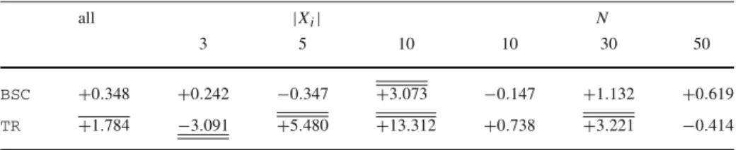
Table 5 Difference between the meanρderived by theCCmethod and that derived by the other methods

all |X_i| N

3 5 10 10 30 50

BSC +0.348 +0.242 −0.347 +3.073 −0.147 +1.132 +0.619 TR +1.784 −3.091 +5.480 +13.312 +0.738 +3.221 −0.414

the case of |X

|=5, the probability that such a ρ becomes larger than 0.862 is 3%. Thus, it can be said that although estimation accuracy is degraded from the |X

|=10 case, fully precise orders are estimated. However, in the | X

|= 3 case, the probability that ρ for random orders will become larger than 0 . 650 is about 27%. For such short orders, it could not to confirm whether fully appropriate orders could be estimated or not. In short, all three methods work well when the sample orders were sufficiently long.

We next examined paired t-tests to check for differences among these methods. Table 5 shows the t-values for the difference between means of ρ derived by the target CC method and those derived by the other methods. The positive t-values indicate the inferiority of the CC. The single-overline and double-overline (single-underline and double-underline) indi- cate that the compared methods are superior (inferior), and that the difference was statistically significant at the levels of 5% and 1%, respectively. In summary, the CC and the BSC were comparable, and the TR was superior to the other two. We next analyze these results more carefully.

Discussion on experimental results We first observed the relationship between the CC and BSC methods. In Sect. 3.2, these two methods are almost equivalent in terms of their mathematical formulation except in terms of their objective functions, Eqs. 2 and 3; the former is the sum, while the later the product of Pr[x

x

|x

, x

]. According to the results in Table 3, the performances on estimation were approximately equal. Further, according to the statistical test (the first row of Table 5), the significant differences are not observed in almost all the cases. We therefore would be able to analyze the properties of Cohen’s ordering model by referring those of the Babington Smith (BS) model.

We here note two known properties of the BS model. First, the orders derived from this

model violate Arrow’s Condition I. For example, suppose three objects, x

, x

, and x

, with

probabilities Pr [ x

x

] = 0 . 6, Pr [ x

x

] = 0 . 1, and Pr [ x

x

] = 0 . 9, respectively. When sorting objects { x

, x

} , the BS model leads to the order x

x

because Pr [ x

x

] = 0 . 6 is the maximum among possible orders. However, for { x

, x

, x

} , the order x

x

x

is selected because the probability is maximized at Pr[x

x

x

] = 0.324/Z , where Z is a normalization constant. Accordingly, the order of x

and x

depends on the other object, x

. This phenomenon is the case in terms of Cohen’s ordering model. In the case of a Thurstone model, Arrow’s Condition I is not violated; all the objects in X

are sorted according to r ˆ ( x

) , which depends only on x

.

Second, in the BS model, it is assumed that ordered pairs of objects are independently gen- erated. Based on the BS model, an order for given X

is generated as follows: For every object pair x

and x

in X

, either x

x

or x

x

is independently chosen with the respective prob- abilities Pr [ x

x

] and Pr [ x

x

] . If the generated ordered pairs do not violate transitivity and can be integrated into one consistent order, the integrated order is generated; otherwise these ordered pairs are all abandoned and re-generated. This process is repeated until a con- sistent order is generated. As described above, this model strongly assumes independence among the ordered pairs. This independence would be assumed in Cohen’s model, too. On the other hand, in a Thurstone model, scores of each object are assumed to be independently generated; thus, the independence assumption among object pairs is less influential.

We then turn to our main goal of these experiments, the comparison of the CC and TR methods. According to Tables 3 and 4, the TR method is generally more effective than the CC. We consider that the advantages of the TR method can be explained as follows. First, as described in Sect. 3.1, the task and the method of Cohen et al. postulate Arrow’s Condition I, whereas their ordering model violates this condition. Such contradiction is not seen in our TR method. We consider this difference evidence of the overall advantage of the TR.

The other cause originates from the fact that an ordering model of the CC more strongly assumes independence among the ordered pairs. This hypothesis would be supported by the experimental results in Table 5. The CC method is superior when the length of the sam- ple orders, | X

| , is short. However, in accordance with the increase of | X

| , the TR method becomes superior. This result is particularly contrasted with the fact that no clear difference was observed between the two methods in terms of changes in the number of examples, N . When | X

| is short, the number of pairs satisfying the transitivity property are fewer, so the independence assumption among pairs is relatively satisfied. However, in correspondence with the increase of | X

|, the independence assumption is more frequently violated. The longer the length of orders becomes, the more advantageous the TR method is.

Finally, we show an additional experimental result. The CC method adopted a greedy

search for finding the order that maximizes the criteria (Eq. 2), so the optimal solution may

not be acquired. Thus, we investigated the difference between the result derived by the greedy

search in Table 2 and the optimal result derived by the exhaustive search. The t-value of the ρ

derived by the optimal search minus the one derived by the greedy search is − 2 . 273. Surpris-

ingly, the ρ derived by the greedy search is significantly better at the level of about 1%. This

result indicates that finding the order so that winners in pairwise comparisons win in the total

order is not equivalent to finding the orders totally concordant with sample orders. This result

enhances the difference between the goal of a Cohen’s task and that of a supervised ordering

task. Note that we cannot clearly explain the above advantage of the greedy search, but can

present one hypothesis. With regard to the sequential selection of the most preceding objects,

the ordering model of the greedy search is not a pure BS model. This sequential process can

be seen in a Plackett–Luce model (Plackett 1975, Marden 1995), and this model does not

violate Arrow’s Condition I. We consider that sequential selection resulted in comparatively

fewer violations of Arrow’s Condition I, and made the greedy search more advantageous.

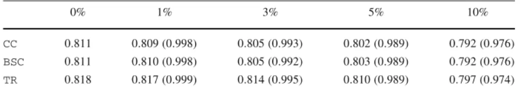
Table 6 The means ofρfor the example sets with order noise

0% 1% 3% 5% 10%

CC 0.811 0.809(0.998) 0.805(0.993) 0.802(0.989) 0.792(0.976) BSC 0.811 0.810(0.998) 0.805(0.992) 0.803(0.989) 0.792(0.976) TR 0.818 0.817(0.999) 0.814(0.995) 0.810(0.989) 0.797(0.974)

Table 7 The means ofρfor the example sets with attribute noise

0% 1% 3% 5% 10%

CC 0.811 0.805(0.992) 0.798(0.984) 0.795(0.980) 0.778(0.960) BSC 0.811 0.806(0.993) 0.798(0.984) 0.795(0.980) 0.779(0.960) TR 0.818 0.815(0.996) 0.811(0.992) 0.800(0.978) 0.776(0.948)

4.1.3 Experimental results on artificial data with noise

We next tested the robustness of our method against the two types of noise. One is the noise caused when two adjacent objects are randomly permutated. In Table 6, we show the means of ρ in the example with a 0% to 10% noise level. The noise level is the ratio of the number of permutated adjacent pairs to the total number of adjacent pairs. The other is the noise that attribute values flip to another value. Table 7 shows the means of ρ in the example sets with a 0% to 10% noise level. The ratio of the ρ to the 0% case is shown in parentheses.

Overall, in terms of robustness against noise, the performance in the case of all the methods was degraded to the same degree relative to the increasing level of noise.

4.2 Experiments on real data

To test the performance of supervised ordering methods on real data, we applied the CC and the TR to real data from the questionnaire survey of preferences in sushi, which were used for the tasks of collaborative filtering (Kamishima 2003) and clustering (Kamishima and Fujiki 2003).

We asked each respondent to sort 10 objects (i.e., types of sushi) according to his/her pref- erence. Such a sensory survey is a very suitable topic for analysis based on orders. The objects were randomly selected from 100 objects according to their probability distribution, based on menu data from 25 sushi restaurants found on the WWW. For each respondent, the objects were randomly permutated to cancel the effect of the display order on their responses. The total number of respondents was 1039. We eliminated the data obtained within a response time that was either too short or too long. Consequently, data for 1025 respondents was extracted. In Table 8, we show the attributes of the objects. The first and second attributes are categorical, the others numerical. These numerical values are discretized by dividing the ranges between the maximum and the minimum into five bins of equal width. In contrast to the case of artificial data, for this data set we could not know true orders. We therefore calculated the empirical error; that is, the ρ between a sample order, O

, and an estimated one, O ˆ

.

To select the proper attribute sets, we examined all combinations of attributes, and the best

result was obtained when eliminating the 6-th attribute. We thus show the result using the

1-st through the 5-th attributes. The means of ρ by performing the LVO test were 0.415 for

Table 8 Attributes of objects (sushi)

No. Descriptions |vl|

1 Style of the sushi: hand-shaped or rolled 2

2 Category of the sushi (e.g., blue fish, vegetables,. . .) 12

3 Heaviness or oiliness of the taste of sushi 5

4 Frequency with which the respondents eat the sushi 5

5 Normalized prices of the sushi 5

6 Frequency with which sushi restaurants supply the sushi 5

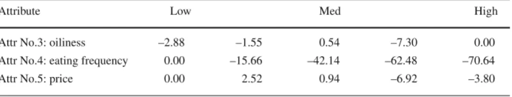
Table 9 Weights of the model learned by theTRmethod

Attribute Low Med High

Attr No.3: oiliness –2.88 –1.55 0.54 –7.30 0.00

Attr No.4: eating frequency 0.00 –15.66 –42.14 –62.48 –70.64

Attr No.5: price 0.00 2.52 0.94 –6.92 –3.80

the CC and 0 . 409 for the TR. These performances appear degraded in comparison with the results on noiseless artificial data, because the performances are measured by using empirical errors that include variations of samples in addition to true errors. According to Eq. 1, the probability that the ρ between the random and the sample orders becomes larger than 0.409 is about 12 . 1%. Thus, the estimated orders are clearly better than the baseline results; i.e., better than the random orders. We consider this level of performance to be sufficient for use in the analysis of preference data. The t-value for the differences between the ρ is + 1 . 532, which indicates that the CC appeared to outperform, though the difference was not significant even at the level of 5%. We observed an advantage of the TR method in the results on artificial data when the length of sample orders was sufficiently long, but no such advantage was found in this result. We suppose that the comparison between empirical errors tended to be affected by a higher level of noise, and the difference became less clear.

Finally, further analysis can be performed by observing the estimated orders and other related data. Table 9 summarizes the weights, w, associated with each of the attribute values of the third, fourth, and fifth attributes. These weights of the regression models are learned by the TR. The smaller the weight of the attribute value, the more preferred the sushi. Based on these weights, rather oily, though not the most oily, types of sushi are preferred. The respondents preferred the types of sushi they ate most frequently. Expensive, but not the most expensive, types of sushi tended to be preferred. Another example of the result of such analysis is this: because the ρ of my (the first author Kamishima’s) preference order is 0.564, it can be concluded that my preference in sushi is the moderately typical type.

5 Conclusion

In this paper, we describe a new learning task and present its solution method: Thurstone

Regression. We applied this method to both artificial and real data, respectively, and analyzed

the experimental results. The results revealed that all the methods can result in placing objects

in the proper order, provided that the sample orders are sufficiently long. The advantages of the TR over the CC become clearer in correlation with increase in the length of sample orders. We articulate the hypothesis that this difference is brought about by the independence assumption among object pairs and/or the violation of Arrow’s Condition I, and showed some rationales for this hypothesis.

We plan to extend the TR method to deal with numerical attributes, and/or to adapt it to non-linear models. We found that the factor | X

|/| X

| affects the estimation performance, and intended to investigate this aspect further.

Acknowledgements This work is supported by the grants-in-aid 14658106 and 16700157 of the Japan society for the promotion of science.

References

Agresti A (1996) Categorical data analysis. Wiley

Anderson JA, Philips PR (1981) Regression, discrimination and measurement models for ordered categorical variables. J R Stat Soc (C) 30(1):22–31

Arnold BC, Balakrishnan N, Nagaraja HN (1992) A first course in order statistics. Wiley Arrow KJ (1963) Social choice and individual values, 2nd edn. Yale University Press

Babington Smith B (1950) Discussion on professor ross’s paper. J R Stat Soc (B) 12:53–56, (A. S. C. Ross, Philological Probability Problems, pp 19–41)

Cohen WW, Schapire RE, Singer Y (1999) Learning to order things. J Artif Intel Res10:243–270

de Condorcet M (1995) On constitution and the functions of provincial assemblies (1788). In: McLean I, Urken AB (eds) Classics of social choice, The University of Michigan Press, chap 7, pp 113–144 Fligner MA, Verducci JS (1990) Posterior probabilities for a consensus ordering. Psychometrika 55(1):53–63 Hayashi C (1952) On the prediction of phenomena from qualitative data and the quantification of qualitative

data from the mathematico-statistical point of view. Ann Inst Stat Math 3:69–98

Herbrich R, Graepel T, Bollmann-Sdorra P, Obermayer K (1998) Learning preference relations for information retrieval. In: ICML-98 Workshop: text categorization and machine learning, pp 80–84

Joachims T (2002) Optimizing search engines using clickthrough data. In: Proceedings of the 8th international conference on knowledge discovery and data mining, pp 133–142

Kamishima T (2003) Nantonac collaborative filtering: Recommendation based on order responses. In: Pro- ceedings of the 9th International conference on knowledge discovery and data mining, pp 583–588 Kamishima T, Akaho S (2004) Filling-in missing objects in orders. In: Proceedings of the IEEE International

conference on data mining

Kamishima T, Fujiki J (2003) Clustering orders. In: Proceedings of the 6th International conference on dis- covery science, pp 194–207, [LNAI 2843]

Kendall M, Gibbons JD (1990) Rank correlation methods, 5th edn. Oxford University Press

Lebanon G, Lafferty J (2002) Crankng: combining rankings using conditional probability models on permu- tations. In: Proceedings of the 19th International conference on machine learning, pp 363–370 Mallows CL (1957) Non-null ranking models. I Biometrika 44:114–130

Mannila H, Meek C (2000) Global partial orders from sequential data. In: Proceedings of the 6th International conference on knowledge discovery and data mining, pp 161–168

Marden JI (1995) Analyzing and modeling rank data, monographs on statistics and applied probability, vol 64. Chapman & Hall

McCullagh P (1980) Regression models for ordinal data. J R Stat Soc (B) 42(2):109–142 Mitchell TM (1997) Machine learning. The McGraw-Hill

Mosteller F (1951) Remarks on the method of paired comparisons: I—the least squares solution assuming equal standard deviations and equal correlations. Psychometrika 16(1):3–9

Nakamori Y (2000) Kansei data Kaiseki. Morikita Shuppan Co., Ltd., (in Japanese)

Osgood CE, Suci GJ, Tannenbaum PH (1957) The Measurement of meaning. University of Illinois Press Plackett RL (1975) The analysis of permutations. J R Stat Soc (C) 24(2):193–202

Sai Y, Yao YY, Zhong N (2001) Data analysis and mining in ordered information tables. In: Proceedings of the IEEE International conference on data mining, pp 497–504

Thurstone LL (1927) A law of comparative judgment. Psychol Rev 34:273–286