Curvature‑driven Interface Evolution with Volume Constraint
著者 ルダイナ モハマド
著者別表示 Rhudaina Z Mohammad journal or
publication title
博士論文本文Full 学位授与番号 13301甲第4144号
学位名 博士(理学)
学位授与年月日 2014‑09‑26
URL http://hdl.handle.net/2297/40537
Creative Commons : 表示 ‑ 非営利 ‑ 改変禁止 http://creativecommons.org/licenses/by‑nc‑nd/3.0/deed.ja
Numerical Analysis of Multiphase Curvature-driven Interface Evolution
with Volume Constraint
(体積保存条件を満たす複数の界面の曲率による運動の数理解析)
金沢大学大学院自然科学研究科
数物科学専攻
計算科学講座
学 籍 番 号 1123102013
名 前 RHUDAINA Z. MOHAMMAD (ルダイナ・モハマド) 主任指導教員名 KAREL ŠVADLENKA (カレル・シュワドレンカ)
– K. ˇSvadlenka
KANAZAWA UNIVERSITY
Abstract
Numerical Analysis of Multiphase Curvature-driven Interface Evolution with Volume Constraint
Rhudaina Z. Mohammad
The dissertation focuses on two main points. First, we develop a signed distance vector approach for approximating volume-preserving mean curvature motions of interfaces sep- arating multiple phase regions – a variant of the MBO (Merriman-Bence-Osher) thresh- old dynamics. We construct a vector-valued analogue of the signed distance function, which provides the needed subgrid accuracy on uniform grids without adaptive refine- ment; thereby, alleviating the well-known MBO time and grid restrictions. We adopt a variational method employing the idea of a vector-type discrete Morse flow, which al- lows us to easily treat volume constraint via penalization, and even, extend our method to include space-dependent bulk energies and anisotropic energies. We present several numerical tests and computational examples of curvature-driven interface evolutions.
Second, we analyze a penalization method related to the above volume-constrained vari- ational problem – an approximation method that penalizes only the increase in volume.
We present existence and regularity results of the sequence of minimizers of the corre- sponding penalized functional. Without relying on the smoothness of the free bound- ary, we investigate the behavior of these minimizers for sufficiently large penalty values.
Lastly, we prove the existence of a minimizing movement corresponding to our penalized functional and some of its properties.
Dissertation Advisor. Karel ˇSvadlenka, Ph.D.
2010 Mathematics Subject Classification. 53C44, 76T30, 49J40, 35R35
Foremost, my deepest appreciation and sincerest gratitude is due to my research super- visor, Dr. Karel ˇSvadlenka for the support, guidance, and mentorship he has provided me during my years of study at Kanazawa University. His positive outlook, stimulating suggestions, encouragement and the always insightful discussions I have had with him contributed immensely in the completion of this dissertation. I am truly fortunate to have had the opportunity to work with him.
The author also extends her gratitude to the Division of Mathematical and Physical Sciences, particularly to the dissertation defense committee: Dr. Seiro Omata, Dr.
Masato Kimura, Dr. Hiroshi Ohtsuka, and Dr. Katsuyoshi Ohara for their input, suggestions, and valuable comments which definitely helped improve this paper.
This work would not have been possible without the support of the Ministry of Educa- tion, Culture, Sports, Science and Technology (MEXT), Japan. Through its Japanese Government (Monbukagakusho) Scholarship Grant, I have had the opportunity to pur- sue a doctoral degree in Mathematics and learn the culture of mathematical research in Japan. I am equally grateful to my employer, Western Mindanao State University, Philippines for granting me a study leave to fulfill a life’s dream.
I wish to thank my fellow graduate students in the Keisan Floor (2F), NST Hall 5 – those who have moved on and those who are still in the quagmire for sharing their research woes and a glimmer of hope for post-graduation normalcy. Special thanks to our lab’s daisempai, Dr. Elliott Ginder for the coding tips and discussions on the MBO Method, and most especially for his 2-month lockdown advice which eventually helped me iron out and debug my SDV program.
My special thanks are extended to the faculty members of the Mathematics and Statistics Department, Western Mindanao State University for their continued moral support and encouragement – un pasion por las matematicas.
I am particularly grateful for the support and the camarederie given by my friends, for being such cheerleaders and accepting nothing less than completion from me. I may not be able to mention all of you here, but know that, I am truly grateful for your existence in my life and I hold you all dear in my heart.
I would also like to thank the Mitsuhashi family in Yokohama, for accepting me with open arms into their home and treating me as one of their own – of course, in particular, to my bestfriend, Rika for the never-ending support. A big thanks is equally due to my Filipino family in Kanazawa, especially to our daisempai, Kuya Edwin and Dr. Rizalita Edpalina for all the cozy and homey time spent on laughters and music. It would be remiss of me not to offer my gratitude to my good friend, Dr. Betchaida Payot for being a wonderful big sister and an inspiration. Your infectious love for rocks and for the country is growing on me.
To my beloved mother and my three little brothers who grew up to be such lovely gentlemen, thank you for the life-long support, love, and understanding. Last but not the least, I want to acknowledge the efforts of all those who have been my teachers in the past, which in one or another have influenced this work. Above all, I thank God Almighty for the strength and courage He has bestowed upon me to finish this work.
vii
Abstract v
Acknowledgements vii
List of Figures xiii
List of Tables xvii
List of Algorithms xix
1 Introduction 1
2 Overview of Multiphase Mean Curvature Flow 3
2.1 Multiphase Motion by Pure Mean Curvature . . . . 3
2.2 Volume-constrained Interface Evolution . . . . 5
2.3 Numerical Methods on MCF Approximation . . . . 5
2.3.1 Front Tracking Method . . . . 6
2.3.2 Threshold Dynamics . . . . 6
2.3.3 Distance Function-Based Algorithm . . . . 7
2.3.4 Vector-type Threshold Dynamics . . . . 8
2.4 Concluding Remarks . . . . 9
3 A Vector Distance Approach to Multiphase Mean Curvature Flow 11 3.1 Construction of the Signed Distance Vector Field . . . 11
3.2 The Algorithm . . . 13
3.3 Velocity of Interface . . . 14
3.4 Triple Junction Analysis . . . 17
3.4.1 Heat Kernel Convolution of Phase Distance . . . 17
3.4.2 Stability of the Triple Junction . . . 21
3.5 Numerical Results . . . 26
3.5.1 Numerical Computations . . . 26
3.5.2 Error Analysis: Shrinking Circle Test . . . 27
3.5.3 Triple Junction: Stability Test . . . 30
3.5.4 Numerical Examples . . . 32
3.6 Concluding Remarks . . . 33
ix
4 On Volume-preserving Multiphase Mean Curvature Flow 35
4.1 Two-phase Flow under Volume Constraint . . . 35
4.2 Multiphase Flow under Volume Constraint . . . 42
4.3 Numerical Results . . . 43
4.3.1 Analysis of the Penalty Parameter . . . 43
4.3.2 Junction Stability: Double Bubble Test . . . 44
4.3.3 Example: Ten-phase Volume-preserving Flow . . . 46
4.4 Concluding Remarks . . . 48
5 Multiphase Mean Curvature Flow considering Bulk Energies 49 5.1 Introduction . . . 49
5.2 Incorporating Bulk Energies in SDV Method . . . 51
5.3 Numerical Results . . . 54
5.3.1 Rising Bubbles with Equal Volumes . . . 55
5.3.2 Rising Bubbles with Unequal Volumes . . . 55
5.3.3 General Transport Motions . . . 56
5.3.4 Example: Six-phase Volume-preserving Flow with Buoyancy . . . 57
5.4 Concluding Remarks . . . 59
6 Volume-preserving Anisotropic Mean Curvature Flow 61 6.1 Introduction . . . 61
6.2 A Numerical Scheme for Anisotropic Evolution . . . 62
6.3 Numerical Results . . . 63
6.3.1 Shrinking Anisotropic Circle Test . . . 64
6.3.2 Example: Two-phase Anisotropic Mean Curvature Flow . . . 65
6.3.3 Example: Two-phase Volume-preserving Anisotropic Flow . . . 66
6.3.4 An Attempt: 7-phase Volume-preserving Anisotropic Flow . . . 67
6.4 Concluding Remarks . . . 69
7 On Evolutionary Free Boundary Problem with Volume Constraint 71 7.1 Introduction . . . 71
7.2 Existence of minimizer and its properties . . . 73
7.3 Interior Regularity of Minimizer . . . 76
7.4 Regularity of Minimizer up to the Boundary . . . 86
7.4.1 H¨older Continuity up to the Boundary . . . 86
7.4.2 Lipschitz Continuity up to the Boundary . . . 93
7.5 Behavior of the minimizer for largeλ . . . 106
7.6 Construction of Minimizing Movement . . . 109
7.7 Concluding Remarks . . . 113
A Reference Vectors: Its Construction and Properties 115 B Expansion of Scalar Signed Distance Function 117 C A Junction-based Signed Distance Vector Approach 119 D Gaussian Function: Some Useful Integrals and Estimates 125
E Calculations involving the Interface Normal 131
F Discrete Morse Flow Method 135
G Multiphase MBO Method considering Bulk Energies 137
H Notations and Preliminaries 143
Bibliography 147
2.1 An illustration of a k-phase configuration of domain Ω. . . . 3 2.2 Thresholding the diffused solution (black) of the characteristic function
(blue) reverts to the same characteristic function causing MBO to get
“stuck”. . . . 7 2.3 Assigning corresponding reference vectors to each phase region. . . . 8 3.1 A 4-phase configuration (top left); the reference vectors pi ∈R3 (bottom
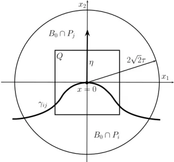
left); and its corresponding signed distance vector field withε= 16 (right). 12 3.2 Setting up interface γij in the new coordinate system. . . 14 3.3 Approximating phase region S by its corresponding tangent wedge Σ. . . 18 3.4 Setting up the triple junction in the new coordinate system. . . 21 3.5 Triangulating domain Ω = [0,1]×[0,1] into 32 nearly uniform elements
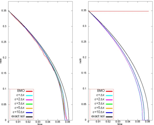
(black) with 22 nodes (blue). . . 27 3.6 Evolution of the radius of a circle generated via MBO (red) and SDV
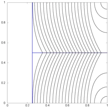
method (non-red) on a 40×40 mesh with ∆t = T /32 (left) and ∆t = T /256 (right) versus the exact solution (black). . . 29 3.7 Evolution of the initial T-junction (blue) via SDV method and its under-
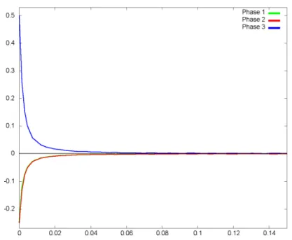
lying interface network at different times (black). . . 30 3.8 Transport velocities at y= 0.47,0.49,0.505,0.55 (left) and interface pro-
file at time t = 50∆t (right) of the SDV numerical solution (colored) versus the constantly transported stable solution (black). . . . 31 3.9 Relative error plot of the phase interior angle measures at the triple junc-
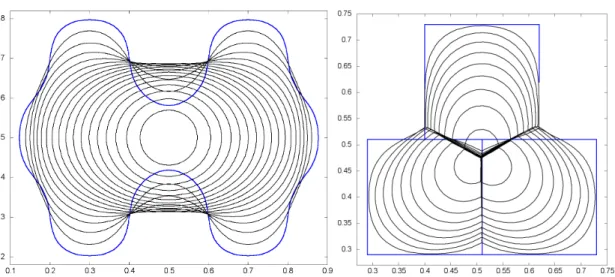
tion for the first 100 time steps. . . 32 3.10 An example of a two-phase (left) and four-phase (right) mean curvature
evolution generated via SDV method. . . . 33 4.1 Evolution of radii (left) for varying penalties % (colored lines) and exact
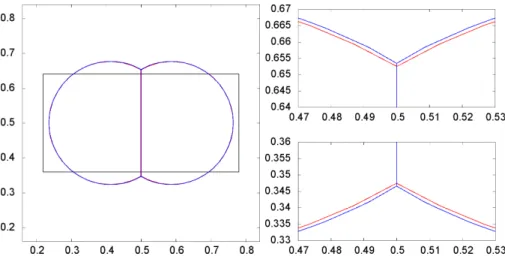
solution (black line). A closer look at the evolution of smaller circle (right) for timet≥0.022 where penalties%= 10−6, . . . ,10−9 overlap. . . 44 4.2 Three-phase initial configuration (left in black); its numerical (blue) and
exact (red) stationary solution. A closer look at the interface network near the triple junctions (right). . . 45 4.3 Relative error plot of the phase interior angle measures at junctionJ1 for
the first 160 time steps. . . 46 4.4 Initial 10-phase configuration (top left); its evolution after ∆t= 2.5×10⁻⁴
(top center) and at different times; and its stationary solution (bottom right). . . 47
xiii
5.1 The motion of two split bubbles of equal volumes (in a three-phase setting) in liquid-filled container with bulk energy density f = 10y (ω1 = ω2 = 2∆)xat different times (left) and the plot of their speed versus time (right). 55 5.2 The motion of two split bubbles of different volumes (in a three-phase
setting) in a liquid-filled container withω1 =ω2 = 2∆xat different times (left) and the plot of their speed versus time (right). . . 56 5.3 The volume-constrained motion of a gas-liquid interface with liquid bulk
energy f = 50(x+y) in the h1,1i-direction (left) and its speed versus time plot (right). . . 57 5.4 Initial 6-phase configuration (top left) and its volume-preserving mean
curvature evolution with zero gas bulk energies and liquid bulk energy f = 25y under volume penalty % = 10−6 with time step size ∆t= 10−3 at different times. . . 57 5.5 A closer look at the first evolution of the rising double bubble (left) and
the two phase regions initially attached to the boundary floor (right). . . 58 5.6 A closer look at the evolution of the interface forming a four bubble link. 58 6.1 Evolution of the radius of an anisotropic circle evolved using φ-MBO
scheme (red) and SDV method (non-red) on an 80×80 (left) and 160×160 (right) mesh resolution with time step size ∆t=T /64 and ∆t=T /128, respectively. . . 64 6.2 Anisotropic mean curvature evolution of a circle via SDV method under
anisotropic energies φ1 (a= 5.5, b= 4.5) andφ2 (a= 0.20). . . 65 6.3 Anisotropic mean curvature evolution of a circle via SDV method under
anisotropic energies φ3 (σ= 10−12,m= 101) andφ4. . . 66 6.4 Volume-preserving SDV evolution driven by anisotropy φ2 with a= 0.20
(top) and φ4 with parameters n = 8, m = 101, σ = 10−12, e0 = h0,1i (bottom). . . 67 6.5 Volume-constrained evolution of a circle via SDV method driven by anisotropy
φ1 (a= 5.5, b= 4.5) under penalty paramter%= 10−6. . . 67 6.6 Initial 7-phase configuration (top left); its volume-preserving anisotropic
evolution after one time step ∆t= 5.0×10⁻⁴ (top center); at t= 10∆t (top right); at t = 100∆t (bottom left); at t = 200∆t (bottom center);
and its stationary solution (bottom right). . . 68 7.1 The subsets of domain Ω which form the five cases in consideration. . . . 104 A.1 Examples of Regular Simplices . . . 115 B.1 Setting up∂S in the new coordinate system. . . . 117 C.1 An example of a 3-phase junction-based signed distance vector field. . . . 120 C.2 Construction of the junction-based signed distance vector. . . 120 C.3 Evolution of a 3-phase smooth interface via junction-based SDV scheme
att= 0,10∆t,80∆t,300∆t. . . 123 C.4 Junction-based SDV: Shrinking Triple Bubble Problem . . . 124 G.1 Setting up interfaceγij in the new coordinate system. . . 137
G.2 Initial three-phase configuration (black in bold) and its volume-preserving mean curvature evolution considering bulk energies e1 = e2 = 0 and e3 = 150y with prescribed contact angles: 180◦−60◦−120◦ (left) and 180◦−120◦−60◦ (right) at different times. . . 141
2.1 A Summary of Numerical Methods for Mean Curvature Flow . . . 10
3.1 MBO Method: Errors for varying mesh-time configurations . . . 28
3.2 SDV Method (ε= ∆x): Errors for varying mesh-time configurations . . . 28
3.3 SDV Method (ε= 2∆x): Errors for varying mesh-time configurations . . 28
3.4 SDV Method (ε= 5∆x): Errors for varying mesh-time configurations . . 28
3.5 DFDGM (ε= 1.0): Errors for varying mesh-time configurations . . . 29
4.1 Double Bubble: Phase Volumes under penalty parameter%= 10−6. . . 45
4.2 Double Bubble: Contact Angle Measures at the Triple Junctions . . . 45
4.3 10-phase Flow: Phase Volumes under penalty parameter %= 10−6. . . 47
4.4 SDV Method in comparison to other MBO-variant Algorithms . . . 48
5.1 6-phase Flow: Phase Volumes under penalty parameter%= 10−6. . . 59
xvii
2.1 Multiphase MBO Algorithm . . . . 7
2.2 Vector-type Threshold Dynamics . . . . 9
3.1 Signed Distance Vector (SDV) Method for Pure Multiphase MCF . . . 13
3.2 SDV Method for Pure Multiphase MCF via Minimization . . . 26
3.3 Steepest Descent Method . . . 27
4.1 Two-phase Volume-preserving SDV Method . . . 39
4.2 Multiphase Volume-preserving SDV Method . . . 43
5.1 Multiphase SDV Method with Volume Constraints and Bulk Energies . . 54
6.1 Two-phase SDV Method for Volume-preserving Anisotropic Flow . . . 63
G.1 MBO Method for Multiphase MCF considering Bulk Energies . . . 138
xix
yo gusta con el matematica . . .
Introduction
The bulk of the present thesis is geared towards developing a scheme for multiphase curvature-driven interface evolutions with volume constraint. By “curvature-driven”, we mean that each point of the interface (separating multiple phase regions) moves with a normal velocity equal to a function of its mean curvature. This type of evolutionary problems often appear in differential geometry and analysis (e.g., study of minimal surfaces), and in a variety of applied problems (e.g., crystal or grain growth, phase transitions, flame propagation, image processing).
The most fundamental problem is thepure mean curvature flow, where the normal ve- locity is given by mean curvature. Under such motion, interfaces contract smoothly to enclose zero volume in finite time. To preserve these phase volumes, the average curva- ture over all interfaces is added to the normal velocity, which regularizes the flow. Such volume-preserving mean curvature flow often appears in applications where physical sys- tems (e.g. soap bubbles, droplets, cell structures) evolve to minimize its surface energy while preserving mass. This is also of interest in image processing where smoothing without shrinkage is desired to preserve significant image features.
Due to its theoretical and practical interest, a variety of computational techniques for mean curvature flow have been proposed. Of particular interest is the MBO threshold dynamics [68] where the characteristic function of each phase region is diffused and sharpened separately (taking the 12-level set as the interface). Such level set approach allows the method to naturally handle complicated topological changes and does not require explicit calculation of mean curvature. Its major drawback, however, is its time and grid restrictions on nonadaptive meshes. To address this issue, Esedoglu et al.[36]
suggested using the signed distance function, in place of the characteristic function.
This provides the needed subgrid accuracies on a uniform mesh to accurately locate the interface and proceed the evolution without stagnation.
Volume-preserving motions can also be produced by thresholding at the level set which preserves the prescribed volume [85]. Unfortunately, this cannot be easily extended to the multiphase case, since average mean curvature of each interface varies, causing inter- faces to overlap or create vacuums. To resolve this issue, ˇSvadlenka et al.[94] proposed a vector analogue of the original MBO scheme using a variational approach to solve the vector-valued heat equation and treat the volume constraint via penalization. How- ever, due to the inherent MBO time and grid restrictions, a temporary and localized refinement is introduced in the algorithm.
1
In this thesis, we are interested in two main points. First, we introduce a signed dis- tance vector modification to the MBO threshold dynamics – a scheme that benefits the main features of its predecessors whilst resolving their key issues. To be precise, we develop a method for realizing volume-preserving multiphase mean curvature flow that (1) naturally handles changes in topology, (2) incorporates interfacial distances in order to alleviate the well-known MBO time and grid restrictions, and (3) set up in a vector- valued fashion to cater any multiphase configuration and easily treat volume constraints using a variational approach via penalization. Using such vector variational scheme, we extend our method to include space-dependent bulk energies and anisotropic energies.
The vector analogue of the scalar signed distance function is mathematically appealing since it may provide hint on characterizing multiphase mean curvature flow by interfacial distances as in [8, 41]. It also implicitly contains geometric information of the interface, which defeats the purpose of localized refinement in [94].
Second, we analyze a penalization method related to the above volume-constrained vari- ational problem. In particular, we consider the problem of successively minimizing the functional R
Ωh−1|u−un−1|2 +|∇u|2 over all nonnegative functions u ∈ H1(Ω) whose set of positive values have Lebesgue measure equal to|{u0>0}|for a given nonnegative Lipschitz function u0 ∈ H1(Ω)∩L∞(Ω) and time step size h > 0. We use an approx- imation method that penalizes only the increase in measure of the set {u > 0}. We prove the existence and regularity of the sequence of minimizers and investigate their behaviors for sufficiently large penalty value λ. Without relying on the smoothness of the free boundary, we show that the measure of the set{u >0}adjusts to its prescribed value providedλis large enough; hence, the solution to the original problem is attained without having to takeλto infinity. To end, we construct a minimizing movement and show some of its properties.
The thesis is organized as follows. We start with an overview of the pure multiphase mean curvature flow in Chapter 2. In Chapter 3, we construct a vector analogue of the signed distance function (Definition 3.1) and show that this vector distance-based scheme moves the interface according to its mean curvature (Theorem 3.3) and sta- bly imposes symmetric junction angles (Theorem 3.7). The succeeding three chapters extend our method to include volume constraints (Chapter 4), space-dependent bulk en- ergies (Chapter 5), and anisotropic energies (Chapter 6). We present several numerical tests and computational examples of these curvature-driven interface evolutions. Lastly, Chapter 7 presents theoretical results on a penalization method for an evolutionary free boundary problem with volume constraint.
Overview of Multiphase Mean Curvature Flow
The present chapter provides an introduction to pure multiphase mean curvature flow.
In addition, we present previous works on numerical approximation of mean curvature flow highlighting their essential features and key issues in relation to volume preservation and the multiphase case, from which, we build the motivation for this study.
2.1 Multiphase Motion by Pure Mean Curvature
Consider a partition ofRN =P1∪P2∪ · · · ∪Pk intokphase regionsPi ⊂RN of positive Lebesgue measure. Define a collection Γ := S{γij :i, j= 1,2, . . . , k} of hypersurfaces inRN whereγij =γji denotes the interface separating phases Pi and Pj, that is, γij = Pi∩Pj =∂Pi∩∂Pj(i6=j).
Ω P1
P3
Pk P4
P2
· · ·
· · · γ12
γ23
γ24
Figure 2.1: An illustration of ak-phase configuration of domain Ω.
The objective is to find a family{Γ(t) :=S
γij(t)}depending on timetsuch that every point x∈γij(t) moves with a velocity
V(x) =−κηij on γij(t), (2.1) 3
where, κ and ηij denotes the mean curvature and unit outer normal from phase Pi to Pj atx, respectively.
Such curvature-driven interface motions often appear in differential geometry and anal- ysis. A number of these literature include local regularity [31, 32]; behaviour of singu- larities [57–59, 95]; uniqueness and existence of generalized solutions in the two-phase setting – using varifolds of geometric measure theory [14], parametric approach [55], and level-set techniques based on the idea of viscosity solutions [24, 40–43]; as well as, existence, uniqueness, and global regularity of interfacial motion with triple junctions [15, 66]. These problems are not only mathematically appealing, but also of practical interest as it often arises in applications in the physical sciences and engineering. To mention a few, grain boundary motion in annealing pure metals [34, 76], phase changes and moving interfaces [39], fluid dynamics [79, 97], evolution of nanoporosity in dealloy- ing [33], and even, in the field of image processing, e.g. image selective smoothing and edge detection [6, 19, 20, 23, 86].
More often than not, this type of interfacial motion is referred to as pure multiphase mean curvature flow since equation (2.1) (as shown in [65, 81]) is derived as the gradient flow for the surface energy functional
E(Γ) =X
i<j
Z
γij
dHN−1 (2.2)
whereHN−1 denotes theN−1-dimensional Hausdorff measure. In this sense, interfaces evolve in order to decrease their surface energies, thereby, playing an important role in the theory of minimal surfaces. In the case when there are three or more phases (k >2), a natural boundary condition arises from the gradient descent for (2.2), known as the symmetric Herring boundary condition which imposes a 120◦−120◦−120◦ angle measures at the triple junction [54].
In the two-phase (k = 2) setting, on the other hand, it was proven that an interface under mean curvature motion contracts smoothly, becoming more and more spherical, as it shrinks to a point and eventually vanishes in finite time [44, 55]. As an example, consider an N-dimensional sphere of initial radius r0, then its mean curvature flow is given by
dr
dt =−N −1
r , r(0) =r0. Hence, the radius of the spherer(t) at timetis
r(t) = q
r20−2(N −1)t,
which implies that the sphere shrinks without changing its shape and disappears at time t=r02/2(N −1).
It is also well-known that two-phase mean curvature motion can be characterized in terms of the distance to the interface [8, 41]. More precisely, letP ∈ RN be the phase region whose boundary∂P coincides with interface Γ. Define the scalar signed distance db:RN →Rby
d(x, t) = dist(x, Pb (t))−dist x,RN\P(t) .
Then, ∇dband ∆dbgives the outer normal and mean curvature, respectively. Moreover, the normal velocity of a point on the boundary at each time is given by−∂d/∂t; hence,b the evolution is characterized by
∂db
∂t(x, t) = ∆d(x, t),b (2.3)
for any x ∈ ∂P(t) = {d(x, t) = 0}, the zero-level set. However, as far as the author’sb knowledge, such a characterization for the multiphase mean curvature flow has yet to be established and remains an open problem.
2.2 Volume-constrained Interface Evolution
Let us consider the case when interfaces evolve by mean curvature while simultaneously preserving the volume of each phase region, that is, |Pi(0)| = |Pi(t)|, ∀t ≥ 0 (i = 1,2, . . . , k), where| · |=LN(·) denotes theN-dimensional Lebesgue measure. This type of motions come in handy in the problem of shape recovery where one achieves smoothing without shrinkage, thereby, preserving important features of the image [29, 87].
This evolutionary problem known as the volume-preserving multiphase mean curvature motion is characterized by the velocity of interface that depends on the lengths and curvatures of all other interfaces. In the two-phase case [17, 90], the velocity of interface Γ is simply given by
V(x) = (−κ+κa)η(x), x∈Γ, where κa =R−
Γ(t)κ(x, t)dHN−1 denotes the average mean curvature along interface Γ.
Adding this extra term κa balances the contraction resulting from the pure mean cur- vature flow and keeps the enclosed volume of the hypersurface constant; thereby reg- ularizing the flow. Under a volume-preserving two-phase flow, a convex hypersurface (interface) remains convex and approaches a constant curvature sphere [9, 45, 56]. Other literature on this problem include existence of global solution starting from non-convex initial hypersurfaces [35] and studies related to constant mean curvature surfaces be- tween parallel places, in particular, stability of cylinders [11] and spherical caps [1]
under volume-preserving mean curvature flow.
Moreover, it was shown that volume-preserving mean curvature flow arises as a singular limit of a nonlocal Ginzburg-Landau equation, in other words, a nonlocal mean curvature motion of interfaces which preserves mass [16, 83]. For this reason, such curvature-driven interface evolution problems often arises in physical systems where the mass of the phase regions remains constant as in capillarity [92], biological cell structure [13], soap films, soap bubbles, and droplets [98].
2.3 Numerical Methods on MCF Approximation
Due to its wide array of applications, an interesting selection of numerical methods for realizing mean curvature flow (MCF) were proposed. This section introduces a number of these algorithms and presents their pros and cons with emphasis on volume preservation and multiphase case.
2.3.1 Front Tracking Method
Front tracking method [17, 63, 67, 69] takes a fundamentally straightforward approach to approximating mean curvature interface evolutions. It involves direct discretization of a parametrization of interface and approximate its motion by explicit computation of the mean curvature and normal direction at each interfacial discrete point, including the average curvature over all interfaces for the volume-constrained case. In the multiphase case, triple junctions are treated separately in order to satisfy the required Herring angle conditions. Moreover, note that all calculations solely are concentrated on the interface.
For this reason, the front tracking method is said to be computationally efficient.
One major drawback of this method is its inability to handle interfaces that cross or have complicated topology. To overcome this problem, one should explicitly detect and treat changes in topology by some selection of rules (e.g. [17] for mean curvature motion of a network of curves). This requires one to enumerate or make assumptions on all possible topological changes that may typically occur. For example, in the two-dimensional case, it is expected (though not proven) that interfaces interact only through junction- junction collisions [66], which translates the problem to detecting junction collisions and perform some form of “numerical surgery” to generate the next interface evolution. For general interface networks, however, this method can be quite impractical to implement, particularly in higher dimensions.
2.3.2 Threshold Dynamics
The threshold dynamics introduced by Merriman, Bence, and Osher (MBO) takes a level set approach for realizing interfacial motions by mean curvature [68]. This scheme is very easy to implement and avoids the complications of the front tracking method – in the sense that it naturally handles topological changes and does not require explicit calculation of the mean curvature and the normal direction.
In the two-phase case, the interface is defined as a boundary of some compact set which evolves through time by alternating two steps: diffusion and thresholding. At each time interval, the 12-level set of the solution of the heat equation (taking the characteristic function of the compact set as the initial condition) approximates the mean curvature evolution of the interface. In fact, this has been extensively shown to converge to the unique viscosity solution of the mean curvature evolution equation [12, 37, 60]
ut−tr
I−Du⊗Du
|Du|2
D2u
= 0 u(0, x) =χΓ(x).
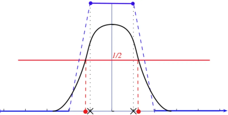
Unfortunately, this algorithm is also known to suffer from a time and grid restriction on nonadaptive meshes [68]. This means that in order to accurately resolve the interfacial motions via an MBO process, one must appropriately choose time step size ∆tso that diffusion proceeds for a long enough time that the half-level set moves at least one grid point. Otherwise, the thresholding step would keep the interface stationary. (For an illustration of MBO stagnation in the one-dimensional case, see Figure 2.2).
In the general multiphase case, the characteristic function of each phase region is diffused and sharpened separately [68, 84], as shown in Algorithm 2.1. Here, the interfaces are
b b
1/2
× ×
Figure 2.2: Thresholding the diffused solution (black) of the characteristic function (blue) reverts to the same characteristic function causing MBO to get “stuck”.
taken as the 12-level sets of all ksolutions, that is,Sk
i=1{ui = 12}. Moreover, the update in the thresholding step maintains the stability of the triple junction imposing symmetric angles [68].
Algorithm 2.1 Multiphase MBO Algorithm
1. Initialization. Set ui0 :=χi, characteristic function of phase Pi (i= 1,2, . . . , k).
2. Diffusion Step. For eachi= 1,2, . . . , k, solve scalar heat equation until time ∆t:
∂ui
∂t (t, x) = ∆ui(t, x) in (0,∞)×RN, ui(0, x) =ui0(x) on {t= 0} ×RN.
3. Thresholding Step. For eachi= 1,2, . . . , k, sharpen the diffused regions by setting ui0 as the characteristic function of{ui(x)≥uj, j= 1,2, . . . , k}.
4. Go back to the diffusion step.
For two-phase volume-preserving motions, Ruuth and Wetton [85] suggested changing the threshold value to 12−12κa(t)
√
π−1∆twhereκadenotes the average mean curvature along the interface. They showed that at this threshold value, the level set preserves the prescribed phase volume. However, this scheme lacks theoretical justification and cannot be easily extended to the multiphase case. This is because each interface yields different average mean curvature, causing interfaces to possibly overlap or create vacuums.
2.3.3 Distance Function-Based Algorithm
To address the time and grid restriction on the MBO threshold dynamics, Esedoglu, Ruuth, and Tsai proposed replacing the thresholding step by a redistancing scheme [36]
where scalar signed distance function is instead, taken as the initial condition in solving the heat equation. Here, the interface is described by the zero-level set of the solution.
Note that the key issue why MBO interface evolutions gets “stuck” lies in the represen- tation of phase regions by the characteristic function. Since the mesh nodal values are
set to either 0 or 1 at the beginning of each time step, the true location of the inter- face is lost and its discrete representation is pushed to the center of the grid. Unlike characteristic functions, signed distance functions implicitly keep geometric information regarding the interface; thereby, providing subgrid accuracies on a uniform mesh and allows one to accurately locate the interface. Hence, this method usually coined as the
“Distance Function-based Diffusion Generated Motion (DFDGM) Algorithm” [34] re- solves the mean curvature motion of the interface without the need for adaptive mesh refinement schemes.
As much as DFDGM method alleviates the time and grid restriction, it also inherits both good and bad points of the threshold dynamics. In particular, it can naturally handle complicated topological changes and does not require explicit computations of the mean curvature. However, as in the MBO method, its approximation to volume-preserving mean curvature flow in the multiphase case still remains in question.
2.3.4 Vector-type Threshold Dynamics
ˇSvadlenka, Ginder, and Omata introduced an interesting spin on the threshold dynamics using vectors, while aimed at realizing multiphase mean curvature flow with volume constraint [94]. Since Ruuth’s approach [84] can not be easily extended to the volume- presering multiphase case, a need to reformat the multiphase MBO algorithm 2.1 arises.
In particular, the authors reformulated the original multiphase MBO scheme in a vector- valued fashion in such a way that volume constraints can be obtained by a constrained gradient flow.
In the two-phase setting (k= 2), observe that representing phase regions by the charac- teristic function is analogous to assigning scalars of equal weights to each phase region, say 1 and−1, the endpoints of a 2-simplex centered at the origin. With this in mind, the authors represented each region in ak-phase configuration, by unit vectors of dimension k−1 pointing from the centroid of a standardk-simplex to its vertices called reference vectors pi (i= 1,2, . . . , k). Figure 2.3 shows an example of a 3-phase representation by reference vectors.
Figure 2.3: Assigning corresponding reference vectors to each phase region.
Taking the reference vector field as an initial condition, the vector-valued heat equation is solved followed by a thresholding step that involves finding the closest reference vector to the solution vector at each nodal point (see Algorithm 2.2).
Algorithm 2.2 Vector-type Threshold Dynamics 1. Initialization. Set u0(x) =pi ifx∈Pi.
2. Diffusion Step. Solve the vector-valued heat equation until time ∆t.
3. Projection Step. Updateu0 by identifying the reference vector closest to solution u(∆t, x), that is,
pi·u(∆t, x) = max
j=1,2,...,kpj ·u(∆t, x).
This redistribution of reference vectors determines the approximate new phase regions after time ∆t, which in turn, defines the new interface network.
4. Go back to the diffusion step.
This method can be thought of as a vector analogue of the original two-phase MBO scheme. In fact, their equivalence can be shown by considering the functions
wi(t, x) = k−1 k
u(t, x)·pi+ 1 k−1
, i= 1,2, . . . , k.
This vector setting allowed the authors to easily treat volume-constrained motions by using a variational approach based on the idea of the discrete Morse flow to solve the vector-valued heat equation and a penalization technique to handle volume constraints.
To overcome the MBO time and grid restriction on nonadaptive meshes, a temporary and localized refinement technique is introduced in the algorithm as follows. Just before the projection step, a record of the interfacial geometry is kept and recalled at the next minimization step. If the interface crosses an element, the geometric information of the interface is used to retriangulate the element and extend the reference vector field, which provides enough subgrid accuracy to proceed to the next evolution.
2.4 Concluding Remarks
We summarize the key features and issues of the above-mentioned numerical methods in Table 2.1. Weighing in both their pros and cons, we think about an MBO-based scheme that takes advantage of the essential features of the above-mentioned modifica- tions whilst resolving their key issues. In particular, our goal is to develop a method for realizing volume-preserving multiphase mean curvature flow that satisfies all six key features listed in Table 2.1. To do this, we adopt the vector approach in [94] in order to cater any multiphase configuration and easily treat volume constraints using a variational approach via penalization. To inherently resolve the MBO time and grid restrictions, we incorporate interfacial distances as in [36] which provides subgrid accuracies without the need for mesh refinement. This requires us to construct a vector analogue of the scalar signed distance function, which in itself, is of mathematical interest, as it suggests a good starting point to characterize multiphase pure mean curvature flow as in [8, 41]
using distances to the interface and derive a partial differential equation analogous to
Table 2.1: A Summary of Numerical Methods for Mean Curvature Flow Features of the Numerical Method Front
Tracking MBO Ruuth’s
Method DFDGM Vector MBO 1. does not require direct calculation of mean
curvature and normal direction
× X X X X
2. handles complicated topological changes × X X X X
3. proceeds the evolution without stagnation X × — X —
4. can be extended to multiphase case — X X X X
5. preserves volume in two-phase case X × X × X
6. preserves volume in multiphase case — × × × X
(Here, “—” means an auxilliary scheme is introduced in the algorithm to resolve the issue.)
the heat equation (2.3). This then, serves as our motivation for designing a signed distance vector approach to approximating volume-preserving mean curvature motions of interfaces separating multiple phase regions, as will be discussed in the succeeding chapters.
A Vector Distance Approach to Multiphase Mean Curvature Flow
In this chapter, we present an MBO-based scheme [68] for treating multiphase mean curvature motions which combines the vector-valued variational approach in [94] with the idea of using interfacial distances [36] to alleviate the well-known MBO time and grid restriction without the need for an adaptive remeshing technique (e.g. [84, 94]). In section 3.1, we construct such signed distance function in a vector setting, which allows us to handle any number of phases. We then modify the MBO Algorithm in section 3.2. In sections 3.3 and 3.4, we formally show that under this scheme, interfaces evolve according to mean curvature flow and that the symmetric Herring angle condition at the triple junction is preserved, respectively. Finally, in section 3.5, we present how we execute our modified MBO algorithm and some numerical tests and examples.
3.1 Construction of the Signed Distance Vector Field
Consider a partition ofRN =P1∪P2∪ · · · ∪Pk intokphase regionsPi ⊂RN of positive Lebesgue measure. Define a collection Γ := S{γij :i, j= 1,2, . . . , k} of hypersurfaces inRN where γij =γji denotes the interface separating phasesPi and Pj, that is,
γij =Pi∩Pj =∂Pi∩∂Pj.
Set up reference vectors pi corresponding to each phase region Pi as unit vectors of dimensionk−1 pointing from the centroid of a standardk-simplex to its vertices. (See Appendix A for details on how these reference vectors are constructed.)
We incorporate distances to each phase region Pi, as follows.
Definition 3.1. Forε >0, we define thesigned distance vectorδε:RN →Rk−1 by:
δε(x) :=
k
X
i=1
1−min
1,di(x) ε
pi,
wheredi(·) :=dist(·, Pi) denotes the usual (Euclidean) distance to phase region Pi.
11
Remark. For any point x∈RN, the following is true for any pair of reference vectors pi and pj (i6=j):
1. IfB(x, ε)∩(Pi∪Pj) =∅, then δε(x)·(pi−pj) = 0.
2. IfB(x, ε)∩(Pi∪Pj)6=∅, then
δε(x)·(pi−pj) = k ε(k−1)
ε−di(x), B(x, ε)∩Pj =∅ dj(x)−ε, B(x, ε)∩Pi=∅ dj(x)−di(x), otherwise.
whereB(x, ε) denotesε-neighborhood of x. Hence,
|δε(x)·(pi−pj)| ≤ k k−1.
Moreover, we note that on interfaceγij, the signed distance vector δε is defined as the sum of reference vectors pi and pj; while on regions away from the ε-tubular neigh- borhood of interface Γ,δεreduces to the reference vectorpi corresponding to its phase locationi.
Example 3.1. In the two-phase case, ε= 1.0 yields the scalar signed distance function (cf. [36]). In this sense, we see that the vector-valued function δε is a multiphase extension of the scalar signed distance function.
Example 3.2. For anyk-phase configuration, the signed distance vector δε approaches the multiphase vector form of MBO (cf. [94]), as ε→0.
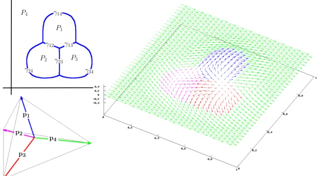
Example 3.3. A more concrete example of the signed distance vectorδε withε= 16 for a four-phase configuration is shown in Figure 3.10.
P3
P2
P1
γ12 γ13
γ23
P4 γ14
γ24 γ34
p3 p2
p1
p4
Figure 3.1: A 4-phase configuration (top left); the reference vectorspi∈R3(bottom left); and its corresponding signed distance vector field withε=16 (right).

![Figure 3.5: Triangulating domain Ω = [0, 1] × [0, 1] into 32 nearly uniform elements (black) with 22 nodes (blue).](https://thumb-ap.123doks.com/thumbv2/123deta/5641130.2003413/50.893.298.644.117.468/figure-triangulating-domain-nearly-uniform-elements-black-nodes.webp)