Bank Lending Strategy in The Stock Market

著者 トリステイヤント 著者別表示 Tristiyanto

journal or

publication title

博士論文本文Full 学位授与番号 13301甲第4313号

学位名 博士（理学）

学位授与年月日 2015‑09‑28

URL http://hdl.handle.net/2297/43826

Creative Commons : 表示 ‑ 非営利 ‑ 改変禁止 http://creativecommons.org/licenses/by‑nc‑nd/3.0/deed.ja

Dissertation

Bank Lending Strategy in The Stock Market

Graduate School of

Natural Science and Technology Kanazawa University

Division of Mathematical and Physical Sciences Course in Computational Science

Student ID No.: 1223102010 Name: Tristiyanto

Chief advisor: Katsuyoshi OHARA

Date of Submission: July 1

, 2015

Abstract

Margin trading is stocks trading using loan leverage from a financial institution; in here we call a bank. It is beneficial for improving liquidity in the market and creating smooth price formation of the stock. However, margin trading has a tendency to escalate the price. As the price of the stocks increases drastically, the authority then raises the minimum margin or minimum collateral to mitigate the risk. Theoretically it will slow down the price movement. Unfortunately, the market reaction result is different. Most of them sell their stocks, so the price then collapses. It was what happen in US great depression in 1929 and lost decade in Japan 1990.

For bank or lender, increasing margin requirements is an effective tool to mitigate the risk.

However, good investors usually also being filtered out by it, as margin requirement only keep investors who have good working capital but, unfortunately, are incompetent to predict good performance investor.

A new method to predict investor bankruptcy in margin trading for the banking industry is suc- cessfully developed. In comparison to the margin requirement that screens investors merely by their capital and collateral, the scope of credit scoring can be extended to include the character, capacity and condition of the trader. Some artificial intelligences to create credit scoring for granting player loan proposals are implemented by comparing multiple discriminant analysis, neural network, decision tree and support vector machine performance then choose the most suitable one. The impact of credit scoring on price movement then is studied to control bubble price movement. Our method can predict investor as bankrupt, surviving and profitable. By clas- sifying the investor into three groups, the bank can manage their loan absorption to profitable and surviving investor.

A new bank strategy for taming the bubble is developed using three methods; these are AI credit scoring, bubble detection and loan adjustment. The loan is delivered base on investor prediction.

When the reserve’s money is running out or bubble condition is detected, bank adjusts the loan parameter so called financing frame. As loan is restricted, the price movement then slightly decreases. After bubble condition or run-out reserve money disappear. The bank can relax the loan.

Various bank’s reserve strategies also are analyzed to find their influence to the price movement.

We performed some simulations to compare a smart bank with a non-smart bank and with static and dynamic reserves. A non-smart bank with a static reserve strategy and dynamic reserve

i

ii strategy will cause a price collapse because the non-smart bank cannot predict investor status so they unable to request early payment to bankrupt investor. Limiting the amount of cash by static reserve will also have a tendency to cause a collapse. When the reserves are gone, the bank is in a dangerous position.

The non-smart bank with dynamic reserve money will generate money creation and on the way building it up the price is collapsed. When the reserves are unlimited, it depends on the total value of the stock market. It is called the money creation as bank print new money to increase the reserve and deliver the money when an investor sells their stock. The dynamic reserve will nurture the development of the price. However, the non-smart bank cannot predict investor status, so they risk to collapsing increase. The impact of the bubble bursting with dynamic reserve money is severer as money creation leads the price to a new level and incompetent non- smart bank explode the bubble.

A smart bank can prevent the collapsing price either using static reserve or dynamic reserve.

When the reserves are limited, the loans will be restricted. Thus, the prices will decrease slightly.

After the reserves are refilled by credit repayments, the bank can relax the loans and the prices will increase. This runs in a continuous cycle. When the bank has large cash deposits, the prices increase steadily. The bank maintains market liquidity by assessing the credit scores of investors.

The smart bank can prevent the bursting price although the reserve is unlimited. Increasing price with smart bank is grounded from good investor financial status. By ability to detect the bubble and predict investor status, the smart bank is able to deliver the loan to profitable and good surviving investor on the right time. Loan will be restricted if investor status is bad or bubble detection is occurred. When condition is safe, bank can relax the loan so market liquidity increases and the price also increases again. Price will move to the new level if investor has good financial status to support it. Thus, smart bank can control money creation to nurture financial development.

Keywords. margin trading, credit scoring, bankruptcy prediction, stock market simulation,

bubble bursting.

Contents

Contents iii

1 Introduction 1

2 Mathematics of Finance 4

2.1 Financial Ratio . . . . 5

2.2 Discriminant Analysis . . . . 6

3 Stock Market 9 3.1 Order Mechanism . . . . 9

3.2 Margin Trading . . . . 13

4 Stock Market Simulation 15 5 Artificial Intelligence 21 5.1 Artificial Neural Network . . . . 21

5.2 Decision Tree . . . . 26

5.3 Support Vector Machine . . . . 27

6 Credit Scoring 30 6.1 Model . . . . 30

6.1.1 Simulation Model . . . . 30

6.1.2 Player Behavior . . . . 35

6.2 Price Discovery . . . . 36

6.3 Credit Scoring . . . . 39

7 Taming the Bubble 45

8 Conclusion 53

Acknowledgement 54

Bibliography 54

iii

Chapter 1 Introduction

Bankruptcy prediction is a challenging topic in business analytics because of the importance of precise and timely strategic business decisions and their impact on the corporation, society and the country and even globally. In the United States, the Great Depression that began 1929 and the 2008 financial crisis when the housing bubble burst and in Japan, the Lost Decade of the 1990s were ignited by the inability to accurately predict bankruptcy [6].

Following these recessions, various regulations were established to ensure the stability of the market and to prevent another collapse [34]. Because buying on the margin is correlated with fi- nancial distress, it can be used as an indicator for detecting an imbalanced financial market [19].

Margin requirements are used to control price volatility and to prevent investors from going into debt to engage in reckless speculation. It is also used to ensure sufficient liquidity in the market that prices are established fairly and smoothly. Relaxing requirements for investing on the mar- gin holds great appeal for the investors, but it is a double-edged sword. Although it increases liquidity, it is also likely to increase volatility [39]. On the other hand, tight requirements re- strict volatility, but the liquidity will be low, because many investors will default. Some of the investors who will be defaulted or file to bankruptcy should be well predicted to manage the risk as instructed on Basel II accord [15]. For a bank or lender, increasing the margin requirements is an effective tool for mitigating risk. However, good investors may also be filtered out since only investors who have sufficient working capital are retained, but, unfortunately, this tool cannot predict which investors will perform well.

In this study, we develop a new method for using credit scoring to predict an investors’ perfor- mance when trading on the margin. Compared to a margin requirement that screens investors merely by their capital and collateral, credit scoring can extend the scope of the evaluation to include the character, capacity and condition of the trader. The simulation presented here was developed from the stock market simulation that was studied by Nakatani et al. [24, 26] and Zhu [43]. The bank agent in that model did not have intelligence and considered only the ratio of debt to working capital. We implemented an artificial intelligence approach to credit scoring for granting loans. We used a statistical method, multiple discriminant analysis [2] and arti-

1

ficial neural networks, decision trees and support vector machines to create our credit-scoring schema.

In the financial industry, credit scoring is well known as a way to predict bankruptcy and thus our research appears to be similar to that of others; however, to the best of our knowledge, there have been no scientific studies of using credit scoring for margin trading. Most of the related research considers ways to predict bankruptcy of companies [12, 14, 21, 23, 28, 35, 42]. How- ever, Wang [38] used an analytical approach to measuring the credit risk for margin trading and calculated the threshold-breaking probability, the default probability and loss given default. In that study, financial ratios were not used to predict bankruptcy, whereas we use the investors’

financial ratios and an artificial intelligence approach to predict the status of each investor. We developed a method for credit scoring that uses three classes (“bankrupt”, “surviving” and “prof- itable”), although most known methods use only two classes (“bankrupt” and “surviving” or good and bad). The “profitable” class is useful for maintaining market liquidity when a bub- ble occurs. Banks can deliver their loans to investors who will help maintain market liquidity.

We consider the impact of credit scoring on price movement and its effect on controlling bub- bles.

We also present a new banking strategy for taming bubbles [25]. Most economists use financial regulations and macroeconomic policies in their attempts to tame the crashes that follow bub- bles. For example, Danthine [9] used capital buffers to mitigate systemic risk and Sornette [36]

developed a method for detecting bubbles and predicting crashes. In our bubble-taming strategy, we use artificial intelligence, credit scoring, bubble detection and loan adjustments. We verified in our cases that if a bank uses our strategy, it can prevent the bubble from bursting.

Various bank’s reserve strategies also are analyzed to find their influence to the price movement.

We performed some simulations to compare a smart bank with a non-smart bank and with static and dynamic reserves. A non-smart bank with a static reserve strategy and dynamic reserve strategy will cause a price collapse because the non-smart bank cannot predict investor status so they unable to request early payment to bankrupt investor. Limiting the amount of cash by static reserve will also have a tendency to cause a collapse. When the reserves are gone, the bank is in a dangerous position.

The non-smart bank with dynamic reserve money will generate money creation and on the way building it up the price is collapsed. When the reserves are unlimited, it depends on the total value of the stock market. It is called the money creation as bank print new money to increase the reserve and deliver the money when an investor sells their stock. The dynamic reserve will nurture the development of the price. However, the non-smart bank cannot predict investor status, so they risk to collapsing increase. The impact of the bubble bursting with dynamic reserve money is severer as money creation leads the price to a new level and incompetent non- smart bank explode the bubble.

A smart bank can prevent the collapsing price either using static reserve or dynamic reserve.

When the reserves are limited, the loans will be restricted. Thus, the prices will decrease slightly.

After the reserves are refilled by credit repayments, the bank can relax the loans and the prices

CHAPTER 1. INTRODUCTION 3 will increase. This runs in a continuous cycle. When the bank has large cash deposits, the prices increase steadily. The bank maintains market liquidity by assessing the credit scores of investors.

The smart bank can prevent the bursting price although the reserve is unlimited. Increasing price with smart bank is grounded from good investor financial status. Ability to detect the bubble and predict investor status makes smart bank able deliver the loan to profitable and good surviving investor on the right time. Loan will be restricted if investor status is bad or bubble detection is occurred. When condition is safe, bank can relax the loan so market liquidity increases and the price also increases again. Price will move to the new level if investor has good financial status to support it. Thus, smart bank can control money creation to nurture financial development.

The rest of this dissertation is organized as follows. In Chapter 1, we briefly describe the back-

ground and the purpose of the research. In Chapter 2, we present mathematical finance that is

used in the research. In Chapter 3, we describe the real world stock market system while, in

Chapter 4, we explain about how our market simulation work. Moreover, we present artificial

intelligence algorithms that are used to develop credit scoring in Chapter 5. The main part, our

results are thoroughly discussed in Chapter 6 for credit scoring and Chapter 7 for taming the

bubble. Finally, we provide remark and conclusion in Chapter 8.

Chapter 2

Mathematics of Finance

The essential idea of credit appraisal is comparing similar characteristic between previously recorded customer behaviour with the new one. If the new proposal has a tendency same with bad group attribute value that default their loan, the proposal should be rejected. If the pro- posal element same with good customer group, then, the loan can be granted. There are two techniques that usually used, these are loan officer judgmental analysis or credit scoring tech- nique [1].

The judgmental technique depends on the expertise and experience of the evaluator. The more expert evaluator can judge not only from the quantitative value of the proposal but also the qualitative value of the person. However, standardizing the evaluator is difficult. Their judge- mental method is inconsistent, subjective and unquantified. These are some weak reasons of this technique. On the other hand, credit scoring provides a quantitative approach for classifying proposal using historical data. Credit scoring can classify with less information being provided.

Only highly correlated data to repayment performance that is needed by credit scoring. The other advantage of this method is replicable easily. Another evaluator can use the same reliable credit scoring method to evaluate other credit proposals with the same performance. The main problem of the credit scoring method is the weakness of the quantitative approach itself. The quantitative approach that can be used are vary from traditional methods such as univariate anal- ysis [23], regression analysis [7] discriminant analysis [2, 7, 23], logistic regression [28] into advanced methods such as neural network [28], genetic programming [7], decision tree [7, 28]

and support vector machine [1, 7, 21, 28].

The simplest credit scoring assessment is univariate analysis. It explores each variable and choose one variable that has the strongest correlation with the target. Miller [23] use total liabil- ity to total asset to show that probability to default increase as liability increase. Altman [2] uses discriminant analysis to predict bankruptcy using multiple variables. His work is well known and widely used in financial industry as his result give good reasoning in approving credit proposal since the variables he used are the firm accounting ratios. We will use discriminant analysis, neural netwrok, decision tree and support vector machine to build credit scoring. Neural net-

4

CHAPTER 2. MATHEMATICS OF FINANCE 5 work, decision tree and support vector machine will be discussed in chapter 5 and discriminant analysis will be explained later after we discuss the following financial ratio section.

2.1 Financial Ratio

Every company produces the financial statement to describe their financial performance. In- vestors use this financial statement to evaluate and justify their investing decision on this com- pany. However, financial statement consists of many items that intercorrelated. Some ratios are developed to make data more meaningful. These ratios are very useful to show the relationship between financial statement data. Not only for analyzing the same company over time but also very helpful to compare among firms performance.

There are many financial ratios to describe the firm financial performance. Altman [2] iden- tified 22 potential ratios that have ability to predict bankruptcy. His further study found that only five ratios that have significant correlation to predict bankruptcy. These ratios are working capital/total assets, retained earnings/total assets, earning before interest and taxes/total assets, market value of equity/book value of total liabilities and sales/total assets [2].

1. (working capital) / (total assets)

Working capital = current assets - current debt. The companies that continuously have operating losses will slice their working capital as their asset is used to cover the losses.

The firms that have positive working capital mean that they can pay their short-term obli- gation.

2. (retained earnings) / (total assets)

Retained earnings = beginning retain earnings + net income or net loss - dividends paid. The ratio determines the maturity of capital firms. The younger firms have a higher tendency to bankrupt than the older firms. Thus, the younger firms will have a low ratio as they have not had the time to accumulate their profit.

3. (earning before interest and taxes) / (total assets)

Fundamentally, this ratio assesses the firms earning power using their assets. It will detect insolvency when the firms cannot utilise their liabilities.

4. (market value of equity) / (book value of total liabilities)

This ratio calculates how much the firm’s asset value can decrease as the market value of equity decline before their debt exceed the asset and the companies become insolvent.

5. (sales) / (total assets)

This ratio measures the assets turnover to generate revenues or sales using their assets. It shows efficiency of the company to utilise their assets to the sales.

As margin trading simulation that is being studied is for individual investor, these financial ratios

cannot be used. Using the same analogy, investor should has individual financial performance.

However, The simulation program also do not populate individual investor characteristics like job, wage, address, age, job duration etc. The simulation program only record investor perfor- mance from four variables, cash, stocks market value, debt and profit. Two important factors to develop financial ratios to evaluate investor are ratio is not hindering other ratio and the ratio can be calculated without being violate computational calculation such as divided by zero. There are eight ratios we propose

1. (market value) / (total assets) 2. (profit or loss) / (total assets) 3. (liabilities) / (working capital) 4. (cash) / (working capital)

5. (market value) / (working capital) 6. (profit or loss) / (working capital) 7. (liabilities) / (total assets)

8. (cash) / (total assets)

2.2 Discriminant Analysis

The multiple discriminant analysis is extended version of linear discriminant analysis (LDA) in- vented by Ronald A. Fisher in 1936 [13] to classify data into more than two classes. LDA works with assumption standard distribution classes or equal classes covariance to search a linear com- bination of variables that best separates two classes. Let Z be a function with linear combination of variables X = { X

, X

, . . . , X

} and coefficients ˜ α = { α ˜

, α ˜

, . . . , α ˜

} as follows:

Z = α ˜

X

+ α ˜

X

+ ··· + α ˜

X

.

Assume that we have N samples { x

,x

, . . . ,x

} by observation, N

of which belong to group 1 and N

to group 2. One noticeable measure to classify the samples is how different are the mean values of Z for the two different groups. Fisher solved it by proposing the followings score function:

S(α ) = (Variance of Z between Groups) (Variance of Z within Groups)

= (α µ

− α µ

)

α

Cα

= (α (µ

− µ

))

α

Cα .

CHAPTER 2. MATHEMATICS OF FINANCE 7 C is a pooled covariance matrix, while C

, C

and µ

, µ

are covariances and means vectors of group 1 and group 2. Given the score function, the objective is to estimate the linear model coefficient α that maximize the score that can be solved by

α = C

(µ

− µ

) C = n

C

+ n

C

n

+ n

.

A new point X is categorized by projecting it onto the maximally separating direction and clas- sifying it as group 1 if

α

=

X − µ

+ µ

2

> log p(G

) p(G

) ,

where p(G

) and p(G

) are the probability of group G

and G

. The result of Fisher’s LDA is equal to least square problems or linear regression classification [41]. It also had been shown by [11].

In 1968, Edward I. Altman discovered a formula that used Fisher’s LDA to predict corporate bankruptcy. His work was developed from William Beaver’s research on bankruptcy prediction, which used univariate analysis of an accounting ratio. Instead of using the t-test to evaluate each ratio, Altman applied discriminant analysis to multiple variables concurrently [2].

He investigated financial data from 66 firms and found 22 potential variables or ratios for pre- dicting from the literature. The variables were grouped into five categories: liquidity, solvency, profitability, leverage and activity. Afterward, those variables were assessed by examining sta- tistical significance impact of each independent variable and inter-correlations among variables.

Prediction accuracy then evaluated before formulated the result. From 22 ratios, 5 ratios were chosen as predictors. The five ratios are X

: (working capital)/(total assets); X

: (retained earn- ings)/(total assets); X

: (earnings before interest and taxes)/(total assets); X

: (market value of equity)/(book value of total liabilities); and X

: (sales)/(total assets). The Z-score formula is Z = 0.012X

+ 0.014X

+ 0.033X

+ 0.006X

+ 0.009X

. A score above 3.0 means that it is un- likely that the company will go bankrupt and a score below 1.8 means that it is likely to do so.

Although the initial test showed that the accuracy is around 72% for the predicting bankruptcy within two years, Altman’s Z-score is the leading model. In 1999, further research by Altman considered more firms and used more recent data and the accuracy was shown to have increased to approximately 80%-90%. The improvement of the Z-score formula has resulted in its use as a bankruptcy prediction tool in other business sectors, such as private firms, non-manufacturers and emerging markets [3].

Altman’s Z-score cannot be used for lending decisions for margin trading because it is difficult

to calculate the Z-score for each investor; in particular, it is difficult to calculate X

, the (market

value)/(total liabilities). If the total liability is zero, then X

will be undefined and if the total

liability is much smaller than the stock market value, X

will be excessively large and will

overwhelm all of the other information. Moreover, for individuals, the variables X

, X

and X

measure almost the same thing, namely, profit per total asset. Although it can be calculated,

the Z-score is not valid for making predictions. However, its principle still can be implemented

to create a credit score for margin trading. Bankruptcy can be predicted by assessing financial ratios which have significant correlation to that outcome.

Our Z -score function is defined by a linear form of eight financial ratios v

, . . . ,v

as fol- lows:

Z = h α ,v i = α

v

+ α

v

+ ··· + α

v

,

where v = (v

,v

, . . . , v

)

and α = (α

,α

, . . . , α

)

. We classify samples into three classes those are bankrupt, surviving and profitable. Then the coefficients α for each class are deter- mined by using Fisher’s LDA. Let µ

be the mean and σ

the standard deviation for each class.

The Z-score for each class can be interpreted to the probability density of investor status as follows:

N

(Z) = 1 q

2πσ

exp

− (Z − µ

)

2σ

.

Hence, we can translate the Z-score function into the AI function f(v) which will be discussed

at Chapter 6.1.1.

Chapter 3

Stock Market

The stock market is a venue where share prices for listed stocks are discovered [33] and owner- ship of shares are exchanged [31]. The stock market shall provide timely and accurate informa- tion on past transactions and current buy and sell order so investors can justified a proper price when entering the market. Another main requirement is the market also should provide liquidity, the ability to buy or sell a stock quickly at a known price. A good market is whether the market could provide no lag in time and price with low transaction cost.

There are two types of stock market, these are primary market and secondary market [31]. Com- panies are acquiring new capital by issuing new stocks and sell it in the primary market. The outstanding stocks then sell in the secondary market. The new stock can be from initial public offering (IPO) or seasoned equity issues. The firm sells their stocks to the public for the first time through IPO while the firm that already has outstanding stocks sells their stock through seasoned equity issues.

The stock market has stricted and complex regulations to ensure transparency and accountability.

Because of that, the members of the stocks exchange are limited. Individual investors who want to do the transaction in the stock market have to join a securities company that already a member of the stock market. The securities company will ask few fees for their services. If investor joins to securities company that is not a member of the stock market, the securities company will put the order to other securities company that has a membership.

3.1 Order Mechanism

The stock market has two major trading systems usually used. It can be one of them or their combination. First is a pure auction market and the other is a dealer market [31]. The pure auction market or an order driven market, is a market that bid and ask or buy and sell orders are matched by an agent that does not have the stocks in a centralized manner. The pure auction

9

market system is also referred to as price driven since spot price is determined by the highest bid price and the lowest ask price.

The dealer market systems or also referred to as quote driven market is a market with at least one individual dealer for one stock provides liquidity for the investors by purchasing and selling the shares for themselves. Ideally, there should be numerous dealer or market maker that will compete against each other to create a fair spot price. They will compete to form the highest bid price when we want to sell and provide the lowest ask price when we want to buy. Thus, the dealer market system is a decentralized trading system.

Based on the operation of the stock exchange, in terms of how and when the share is traded, stocks market is divided into two categories, call market and continuous market [31]. Call market is a batch market system by matching ask and bid price to a single spot price that execute as much as possible the quantity of demand and supply. Usually, call market is used in an opening market. The opening fair price is determined from a queue of order after the market is closed. The continuous market order executes at any time when the market is open either by auction or by dealers. The continuous market operation matches the order from the price and time arrival.

The Tokyo Stock Exchange (TSE) is a double auction continuous market system mixed with the call market system. In the opening market, the TSE uses call market so call itayose method and after the market open, the TSE uses double auction continuous operation so called zaraba method [37]. In Itayose method, the price is defined using these three necessities

1. All market orders must be executed. Market order is buy or sell order with spot price.

2. All limit orders to offer at prices lower than spot price must be executed and bid orders at prices higher than spot price also must be executed. Limit order is buy or sell order by specifying the price.

3. At the spot price, either all buy or all sell orders must be executed completely.

The following table 3.1 illustrates an order book. We will use itayose method to determine the opening price. Aggregated offers start from market order then lowest price to the highest price while aggregated bids start from market order then highest price to the lowest price. The 3 requirements are set to determine the fair price that balances out between aggregated bids and offers.

After the market open, the order transaction now uses double auctions continuous mechanism

or zaraba method. It is called double because the price formations are auction on buy and sell

orders. Zaraba method is the process to match incoming order with the highest priority order

that already in the order book. The order priority is determined by price and time. Market order

is the highest priority. Moreover, The highest price in bids and the lowest in offers have higher

priority over the other. In the same price, priority is decided by arrival time, the earliest has the

highest priority. The table 3.2 shows how the order is executed after the market open.

CHAPTER 3. STOCK MARKET 11 Table 3.1: The Itayose Method

Offer (sell) Price Bid (buy)

Aggregate Quantity Quantity Aggregate

600 Market Order 500

5300 700 752 100 600

4600 1500 751 500 1100

3100 2000 750 1500 2600

1100 300 749 800 3400

800 200 748 2500 5900

Offer (sell) Price Bid (buy)

600 Market Order 500 According requirement (1), market order should be executed first, 500 shares buy orders are matched with 500 shares sell orders at market price leaving 100 shares sell orders

700 752 100

1500 751 500

2000 750 1500

300 749 800

200 748 2500

Offer (sell) Price Bid (buy)

100 Market Order

All market orders, bid orders above spot price and offer orders below spot price are matched, fulfil requirement (1) and (2)

700 752 100

1500 751 500

2000 750 1500

300 749 800

200 748 2500

Offer (sell) Price Bid (buy) Market Order

At spot price, All amount of buy orders, 1500 shares at 750 JPY is matched with 1500 shares sell orders. Leaving 500 shares sell orders.

700 752 100

1500 751

2000 750 1500

749 800

748 2500

Offer (sell) Price Bid (buy) Market Order

Finally, All the requirements are fulfilled.

The opening price is 750 JPY and the or- der book now look like this.

700 752

1500 751

500 750

749 800

748 2500

Table 3.2: The Zaraba Method Offer (sell) Price Bid (buy)

1000 Market Order Currently, the best bid is 2000 shares at 749 JPY and the best offer is 500 shares at 750. The market price now is 750 JPY.

A market sell order arrives at the book for 1000 shares.

800 752

1000 751

500 750

749 2000

748 3000

Offer (sell) Price Bid (buy)

Market Order This new sell market order is matched with the bid highest priority, 2000 shares at 749 JPY. Leaving 1000 shares bid order at 749 JPY. The market price is now 749 JPY.

800 752

1000 751

500 750

749 1000

748 3000

Offer (sell) Price Bid (buy)

Market Order After that, 1000 shares bid order arrives at 751 JPY. It will be matched with the of- fer highest priority 500 shares at 750 JPY.

Thus, the market price increases to 750 JPY.

800 752

1000 751 1000

500 750

749 1000

748 3000

Offer (sell) Price Bid (buy)

Market Order The outstanding 500 shares are now matched with 1000 shares offer at 751 JPY. The market price then increases to 751 JPY. Leaving 500 shares at 751 JPY.

The transaction continuously run this way during the trading hours.

800 752

500 751

750

749 1000

748 3000

CHAPTER 3. STOCK MARKET 13

3.2 Margin Trading

Fundamentally, margin transaction is a credit transaction where the investor only pays some por- tion of the cost and the financial institution will pay the remaining [8]. Margin trading useful for increasing liquidity and fair price smooth formation as margin trading will attract more investor to trade by the help of securities financial firms money. Financial brokerage uses the shares as collateral for the loan. So, when the investor sells their stock they have to pay their loan plus interest. People can leverage their capital to gain bigger profit by buying in the margin. How- ever, it is a double-edged sword that also increases the risk of loss. Minimum margin for TSE market is 30% of transaction value or 300,000 JPY whichever is greater while New York Stock Exchange (NYSE) is 50% of transaction value. Furthermore, maintain margin to be preserved, as fluctuation of the price is at least 20% for TSE and 30% for NYSE.

Currently, The TSE in Japan implements two types of margin trading; the first is standardized margin trading and the other is negotiation based margin trading [18]. The standardized margin trading governs by specific regulation set by the TSE. The TSE defines which share that eligible to trade in margin trading base on their liquidity with particular terms. On the other side, large financial companies usually perform the negotiation margin trading. They freely negotiate the fees and the terms.

Standardized margin trading in Japan was firstly implemented in 1951. Specialized securities financial companies were appointed to provide credit and borrowed shares to stabilize and ex- pand Japan’s securities market within the doubtful period after World War II [18]. As individual investors are less creditworthy, the system tries to offer investing leverage for more individual investors to borrow stocks and funds from securities finance companies easily. This process is identified as a security loan transaction so call taishaku torihiki in Japanese. The standardized margin trading work as follows: investor sends margin order to broker. The broker then checks their order list and stocks portfolio to match the order with other orders for the same stock from other investors. When brokers stocks inventory and the matching process cannot fulfill the mar- gin order from the investor, the broker then contact the securities finance company to fill the gap.

The ordinary loan transaction regulation was relaxed since Japanese the financial big bang in December 1998 [18]. Investors and brokers can negotiate the loan rate and repayment period at will. Thus, negotiation based margin trading then started. However, mostly the players of negotiation based margin trading are institutions rather than the individuals because institutions are more creditworthy to negotiate the contract than the individual. Not only the player, but also capitalization value.

Figure 3.1 describes the margin trading system in the TSE. Just like ordinary stock transaction,

customer should join a securities company to be able do a transaction. For margin trading,

customer opens a special account transaction so call margin account. Margin account is used

to manage stock transaction, loan and client’s collateral. Securities company acts as brokerage

for investor to help transaction in stock exchange, manage stock settlement with clearinghouse

and deal with financial institution like bank or other securities finance firm to provide loan to

Figure 3.1: Margin Trading System in Tokyo Stock Exchange [20]

investor. So, in here, securities company hinders all complicated work from investor. Investors

only know one door to do all the transaction just by open a margin account.

Chapter 4

Stock Market Simulation

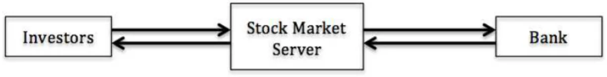
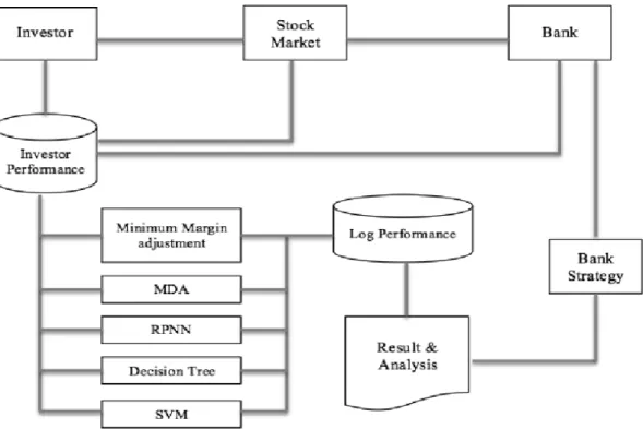
Figure 4.1: Stock Market Simulation

The stock market simulation is developed base on Nakatani [24] and Zhu [43] work. There are three main agent, Investors, stock market server and bank. Investors and bank agent are developed using Java programming language and stock market server using C programming language. Moreover, multiple investors can connect to stock market server to trade. The three of them communicate using TCP/IP. This communication does not allow any loss of data. Any one bit of error will lead one message fail to interpret. We use the followings message format to transmit and receive data.

Data ID: 32 bit signed Integer Data: Depends on the message

The stock market simulation server applies a simplified Tokyo stock exchange rules. At Tokyo stock exchange, the order is accepted on between 8:00 -11: 00 and 12:05 - 15: 00. The market opens at 9:00 - 11: 00 (morning session) and 12:30 - 15:00 (afternoon session). At 8:00 - 9:00 and 12:05 - 12:30, the orders are accepted and processed by itayose method. In the morning ses- sion and afternoon session, the order is processed by zaraba method. We only implements

1. Double auction continuous trading mechanism or zaraba method, so the closing price will become the opening price in the following day.

2. There are two types of order, market order (highest priority) and limit order (lower prior- ity). Limit order can be bid or offer order.

15

3. The tick price is 5 JPY.

4. There are 300 turns time in one day.

5. There is only one type of the stock.

6. The trading unit is 1 share.

7. In one day, there is only one trading session.

We divide the stock market simulation operation into 11 processes, there are login process, order process, order cancellation process, loan process, logout process, order execution process, board information, bank process, loan with credit scoring process and time update.

1. Login process

Every time client connects to the stock market server, server gives the client ID and iden- tifies the client using this ID for any process. The table 4.1 shows the detail of the login process.

Table 4.1: Login Process

Client Server

Message Description Action Description

Login request Request for client ID Login Registra-

tion Send Client ID

Market size in- quiry

Ask how many stock

name that will be traded Send market size Send a number of stock name that will be traded Collateral rate in-

quiry Ask rate of leverage Send collateral rate

Send collateral rate or financing frame

Stock price in-

quiry Ask the initial price Send stock price Send the initial stock price

Send cash Send initial cash Set the client cash Record the client initial Server time in- cash

quiry Ask server current time Send server time Send server current time

2. Order process

The investor initiates order. Investor sends an order to the server then the server register the order to the board list. The table 4.2 describe the message passing.

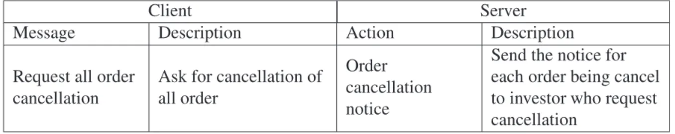
3. All order cancellation process

If player send an instruction to cancel all of his order, server will search all his order and

cancel it from the board list. Server will send notification to the investor for each order

being cancelled. The table 4.3 illustrates the communication.

CHAPTER 4. STOCK MARKET SIMULATION 17 Table 4.2: Order Process

Client Server

Message Description Action Description

Send an order Submit an order Order registration Received order is registered to the board Table 4.3: All Order Cancellation Process

Client Server

Message Description Action Description

Request all order cancellation

Ask for cancellation of all order

Order cancellation notice

Send the notice for each order being cancel to investor who request cancellation

4. Loan process

Investors send loan request to the bank. They send their loan amount proposal and their working capital. Bank checks their remaining loan and loan proposal. If adequate, the loan granted. The table 4.4 describe the process.

Table 4.4: Loan Process

Client Bank

Message Description Action Description

Loan request

Send loan amount proposal and working capital

Financing submitted

Compare the loan proposal and remaining loan of that investor. If sufficient, send the financing. If not, send zero financing

notification.

5. Logout process

If a player send request to logout, Server will cancel all his order and detach him from the server. The table reftab:logout shows the message passing.

6. Order execution process

Order execution is based on double auction continuous method. If there is an execution,

the owner of the order will be notified by a message describes on the table 4.6. If number

of buy order and sell order are the same, both of them are cleared from the board. If not

the same, then there is a remaining order on the board.

Table 4.5: Logout Process

Client Server

Message Description Action Description

Logout request Send instruction to logout

All order cancellation notice

Send notices of all order being cancelled and detach the client from the server.

Table 4.6: Order Execution Process

Server Client

Message Description Action Description

Send execution order information

Send number of shares being executed and the execution price to the owner of the order.

Update client’s portfolio

Client update his stock, cash and order number.

7. Board information

On every turn, the server broadcast information of the board, total remaining loan avail- able and the current time of the server. The table 4.7 shows the message.

Table 4.7: Board Information

Server Client

Message Description Action Description

Send board information

Send all the quantity of the order and the spot price.

Update board information

Client update their information base on current board data Send bank

information

Send total available

loan. Update account Client update his account

Send server time Send current time of

the server. Update time

Client time synchronize with server

8. Bank process

On every turn, bank will send request of repayment to the investor who has due date and bankrupt notification to particular investor. The table 4.8 describes the message.

9. Loan with credit scoring process

If bank credit scoring is activated, when the investor request for loan, the bank will cal-

CHAPTER 4. STOCK MARKET SIMULATION 19 Table 4.8: Bank Process

Bank Client

Message Description Action Description

Send repayment request

After due date and the total loan amount exceeds the total amount available for lending, bank send repayment request to all clients who received the loan.

Repay

Clients repay the loan with their cash if not adequate they sell their stocks at market price

Send bankruptcy notification

If investor cannot pay the loan after the repayment instruction, bank send bankruptcy notification and force the client to logout.

Liquidated and detach

Client sell their stocks at the market price, cancel all order and detach from the program

culate investor credit scoring and judge the credit appraisal from this credit scoring. The table 4.9 illustrates the message.

10. Time update

Client and server program are synchronized by server time. On every turn, server sends

its current time. The table 4.10 shows the message.

Table 4.9: Loan Process with Credit Scoring

Client Bank

Message Description Action Description

Loan request

Send loan amount proposal, shares market value, cash, debt and profit

Financing submitted

Compare the loan proposal and remaining loan of that investor. If sufficient, bank

calculates investor credit scoring, if the score eligible for the loan then bank send financing. If not, send zero financing

notification.

Table 4.10: Time Update

Server Client

Message Description Action Description

Time update Notification for next

turn. Next turn

Client send their

current portfolio

information to the

server and increment

their time

Chapter 5

Artificial Intelligence

5.1 Artificial Neural Network

The artificial neural network is a cellular system that can learn, store and recall its knowledge.

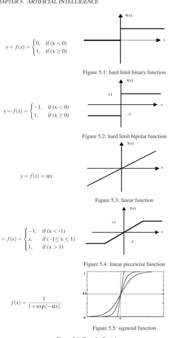
It is constructing by modelling the structure of the human brain. The human brain consists of millions of interconnected neurons that using biochemistry reaction on receiving, processing and transmitting the signal. Information is received by dendrites from the external environment or neighbor neurons. It is then collected and transmitted through axon and dendrites (if over the threshold) to other neurons. Among dendrites, there is a synapse, which can reduce or strengthen the information. On the other hand, the artificial neural network receives information from n inputs. Each input has relative weight than others just like a synapse. The information then is summed and transmitted through processing element called transfer function [10]. The transfer function is a formula to convert the input into output. There are also many types of transfer functions. Examples of various basic of transfer functions are listed below

1. Hard limit

There are two types of hard limit transfer function, binary and bipolar. Binary hard limit transfer function provides output 0 or 1 and the bipolar hard limit produce 1 if input less than 0 or -1 if input greater or equal 0.

2. Linear

Unlike the hard limit transfer function that only provide two output, linear transfer func- tion can provide unlimited output. Linear transfer function is calculate by y = f(x) = α x.

If output equal with input, the function is called an identity function.

3. Linear piecewise

This function only produces linear output between 1 and -1. Otherwise, 1 if input greater than 1 and -1 if input less than -1.

21

4. Sigmoid

The sigmoid transfer function can have any value input x between minus infinity and plus infinity and squashes the output into the range 0 to 1.

The Figure 5.6 shows the transfer functions and their equation.

The artificial neural network can be consisted of one or multi-layer neurons. There are four basic neural network architectures: feed forward, recurrent, symmetrical and asymmetrical [10].

1. Feed Forward

In feed forward neural network, there is no loop node interconnection. It provides a quick response to input.

(a) Single layer feed forward network

In this layered neural network, the neurons are organized in the form of Layers. In this simplest form of a layered network, we have an input layer of source nodes those projects on to an output layer of neurons, but not vice-Versa. In other words, this network is strictly a feed forward or acyclic type. Figure 5.7 illustrates the architecture [10].

(b) Multi layer feed forward neural network

Multilayer feeds forward networks: The second class of the feed forward neural network distinguishes itself by one or more hidden layers. The computation nodes that are correspondingly in the hidden unit are called neurons or units. The function of hidden neurons is intervened between the external input and the network input in some useful manner. The ability of hidden neurons is to extract higher-order statistics is particularly valuable when the size of the input layer is large. The input vectors are feed forward to 1st hidden layer and this pass to the second hidden layer and so on until the last layer i.e. output layer, which gives actual network response.

Figure 5.8 shows the multi layer feed forward neural network architecture [10].

2. Recurrent

A recurrent network differentiates itself from feed forward neural network, in that it has least one feed forward loop. As shown in Figure 5.9 output of the neurons is fed back into its inputs is referred as self-feedback [10]. A recurrent network may have a single layer of neurons with each neuron feeding its output signal back to the inputs of all the other neurons or multi-layer network so the network may have hidden layers or not.

3. Symmetrical

In symmetrical neural network, multiplication result of output of node i with weight i to j is the same with multiplication result of output of node j with weight j to i. Figure 5.11 shows the symmetrical network architecture [10].

4. Asymmetrical

In asymmetrical neural network, multiplication result of output of node i with weight i to j is not the same with multiplication result of output of node j with weight j to i.

Figure 5.12 shows the asymmetrical network architecture [10].

CHAPTER 5. ARTIFICIAL INTELLIGENCE 23

y = f (x) =

( 0, if (x < 0) 1, if (x ≥ 0)

Figure 5.1: hard limit binary function

y = f (x) =

( − 1, if (x < 0) 1, if (x ≥ 0)

Figure 5.2: hard limit bipolar function

y = f (x) = α x

Figure 5.3: linear function

y = f (x) =



 

 

− 1, if (x < -1) x, if ( -1 ≤ x ≤ 1) 1, if (x > 1)

Figure 5.4: linear piecewise function

f (x) = 1

1 + exp ( − α x) .

Figure 5.5: sigmoid function

Figure 5.6: Transfer Function

Figure 5.7: Single Layer Feed Forward Network

Figure 5.8: Multi Layer Feed Forward Network

Figure 5.9: Single Recurent Network Figure 5.10: Multi Recurrent Network

Figure 5.11: Symmetrical Network Figure 5.12: Asymmetrical Network

Figure 5.13: Neural Network Architecture [10]

CHAPTER 5. ARTIFICIAL INTELLIGENCE 25 Artificial neural network (ANN) consists of three layers, input layer, hidden layer and output layer. In the experiment we use eight nodes input layer, five nodes hidden layer and three nodes output layer representing each class, bankrupt, survive and profit. Sigmoid transfer function is used in each node. Each hidden unit computes the weighted sum of its inputs to get a scalar net activation or we call net. net

is a net activation of hidden layer j. It is the inner product of weight of hidden unit and the inputs.

net

=

d i=1

∑

x

w

+ w

=

d i=0

∑

x

w

≡ w w w

xxx,

where i is index unit of input node, j is index unit for hidden layer, d is number of input unit and w

is bias unit. w

is weights at hidden layer j that connect to input layer node x

. Each hidden unit produce an output (y

) as its activation function.

y

.

Similarly, each output node also calculate its net activation based on hidden unit result.

net

=

h

∑

y

w

+ w

=

h

∑

y

w

≡ w w w

yyy,

where k denotes the index of the output node in output layer, h is number of hidden unit and w

is bias unit. Each output node calculate the transfer function with the data from hidden unit result.

z

= f (net

).

A chosen output class is the node with highest score.

max z

.

The fundamental concept of neural networks is that such parameters, weight or bias, can be adjusted so that the neural network exhibits some desired or interesting behavior. Thus, the network can be trained to do a particular job by changing these parameters. One of the learning algorithms that known from its fast performance is resilient propagation. Resilient propagation neural network (RProp) was created by Martin Riedmiller and Heinrich Braun in 1992 [32].

RProp is classified as supervised learning rule for feed forward artificial neural network. RProp uses batch updates to obtain the gradient of each weight. Sign of gradient is used to estimate the direction of weight update. The following is general algorithm of RProp where E(t) = E(w,t) is an error function at time t and w

is weight of neuron ij.

1. Evaluate error after a batch of training examples.

2. Discover the gradient’s direction by identifying sign of gradient of error function

∂wij

and

∂wij

.

3. Take a greater step (η

∆

(t − 1)) than last epoch if sign is the same as the last epoch.

4. If it is different sign as last epoch, it means optimal weight has passed over. Step back and take a smaller step (η

∆

(t − 1)) for next epoch.

Furthermore, different weights need different value of step sizes for update. A step update value

∆

(t) at time t is calculated according to the following recurrence formula:

∆

(t) =



 

 



 

 



η

∆

(t − 1),

if ∂ E(t − 1)

∂ w

∂ E (t)

∂ w

> 0

η

∆

(t − 1),

if ∂ E(t − 1)

∂ w

∂ E (t)

∂ w

< 0

∆

(t − 1), (otherwise), where

0 < η

< 1 < η

.

Weight update (∆w

(t)) then decrease as much update value ( ∆

(t − 1)) if gradient weight is positive (increasing error). On the other hand, weight update (∆w

(t)) is increasing as much update value ( ∆

(t − 1)) if gradient weight is negative (decreasing error).

∆w

(t) =



 

 



 

 



− ∆

(t − 1),

if ∂ E

∂ w

(t) > 0

+∆

(t − 1),

if ∂ E

∂ w

(t) < 0

0, (otherwise).

From the empirical research, the best result is achieved by initial step sizes of 0.1, η

= 1.2, η

= 1.2, η

= 50 and ∆

= 10

.

5.2 Decision Tree

Ross Quinlan invented C4.5 [30] to generate a decision tree using divide and conquer technique.

In order to divide and conquer the data, C4.5 uses information entropy concept. Entropy is exploited to quantify how informative a variable to separate the data. The Entropy of sample S is calculated as follows:

Entropy (S) = − p

log

p

− p

log

p

where p

and p

are proportions of examples of class 1 or class 0 in sample S. Essentially, the entropy evaluates the order (or disorder) in the sample data S with respect to the classes.

It generates 0 (maximal order, minimal disorder) when p

= 0 or p

= 0 and it generates 1

CHAPTER 5. ARTIFICIAL INTELLIGENCE 27 when p

= p

= 0.5 (maximal disorder, minimal order). Gain(S,X

) is described as anticipated reduction in entropy as a result of splitting or sorting on attribute X

Gain(S,X

) = Entropy (S) − ∑

v∈values(Xi)

| S

|

| S | Entropy (S

)

where values (X

) denote the set of all potential values of attribute X

, S

the subset of S where attribute X

has value v and | S

| is the number of observations in S

. The Gain principle was used select upon which attribute to split at a given node. However, when this criterion is applied to determine the node splits, the algorithm favors create leafs on attributes with many distinct values. In order to rectify this, C4.5 implemented normalization and uses the gain ratio criterion, which is described as follows:

Gain ratio (S, X

) = Gain(S,X

) Split Information (S,X

) Split Information (S, X

) = − ∑

k∈values(Xi)

| S

|

| S | log

| S

|

| S | .

5.3 Support Vector Machine

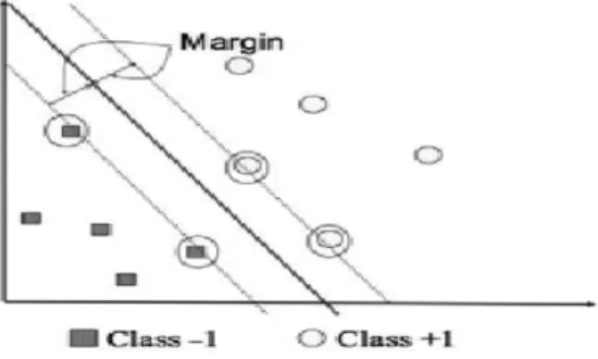
Support vector machine (SVM) firstly invented by Boser, Guyon and Vapnik in 1992 [5] by combining margin hyperplane and kernel method for discriminate two groups data. Margin hy- perplane is used as linear classifier while non-linear data is treated by kernel trick to manipulated domain function into higher dimensional space. The essence of SVM is finding the best hyper- plane as a classifier of two classes in input space, for example, classes +1 and − 1. Look at Figure 5.14, class − 1 is on the left and class +1 is on the right. Classification problems can be translated as an endeavor to obtain hyperplane (line) that separate two groups. The best hy- perplane between those classes can be computed by finding their maximum margin hyperplane.

Margin is the closest distance between two classes pattern.

Figure 5.14: Margin Hyperplane

Training data are symbolized as xxx

∈ R

and class label for each data is noted by y

∈ {− 1, +1 }

for i = 1,2, 3, . . . , l, which l is number of data. Denote by xxx · yyy the dot product of two vectors. It

is assumed that class − 1 and +1 can be separately perfectly by a hyperplane in d-dimensional space R

that is defined as follows:

w w w · xxx

+ b = 0.

Furthermore, positive and negative instances of training data can be written as w w w · xxx

+ b ≥ +1 for positive training data y

= +1, w w w · xxx

+ b ≤ − 1 for negative training data y

= − 1.

Consider two hyperplanes

H

= { xxx ∈ R

| w w w · xxx + b = 1 } and H

= { xxx ∈ R

| w w w · xxx + b = − 1 } . Then the distance between the two hyperplanes is given by

dis (xxx

,H

) = | w w w · xxx

+ b + 1 |

k w w w k = | 1 + 1 | k w w w k = 2

k w w w k , where xxx

∈ H

.

To gain the best hyperplane, we have to maximize the distance 2/ k w w w k . The distance will be maximized if a function τ(w w w) = 1

2 k w w w k

is minimized. The vector w w w and the scalar b can be found by minimizing equation (5.1) with equation constrain (5.2).

min

τ(w w w) (5.1)

y

(xxx

· w w w + b) ≥ 1, i = 1, . . . , l, y

∈ {− 1,+1 } . (5.2) It is so-called quadratic programming problem. Lagrange multiplier then is used to solve this problem. We put g

(w w w,b) = y

(xxx

· w w w + b) − 1 and construct corresponding Lagrangian as fol- lows:

L(w w w,b, α) = τ(w w w) −

l i=1

∑

α

g

(w w w,b)

= 1

2 k w w w k

−

l i=1

∑

α

(y

(xxx

· w w w + b) − 1), α

≥ 0, ∀ i, (5.3) where α

is a Lagrange multiplier with positive value. Optimal value of equation (5.3) can be found by minimizing L by w w w and b and maximizing L by α

. By finding partial derivative L = 0, we get

∂ L

∂ w = w −

l

∑

α

y

x

= 0 (5.4)

∂ L

∂ b =

l i=1

∑

α

y

= 0. (5.5)