宮 崎 大 学 大 学 院 博 士 学 位 論 文
Evaluation of the potential of biodiversity conservation in agriculture-forest mixed landscapes in East Java, Indonesia
(インドネシア東ジャワの森林農地複合景観における生物多様性保全機能の評価)
学 位 授 与
2020年
9月
宮崎大学大学院農学工学総合研究科 資源環境科学 専攻
Yasa Palaguna Umar
Contents
Abstract
Chapter 1. Introduction
1.1. Background: Needs of feasible and effective safeguards for REDD+
1.2. Approaches detecting hot spots from landscape context 1.3. Proposing alternatives to extensive monocultures 1.4. Objective of this study
Chapter 2. Detecting potential biodiversity hotspots for development of REDD+
safeguards based on analyses of land-cover complexity in East Java, Indonesia 2.1. Objectives
2.2. Methods
2.2.1. Study area 2.2.2. Data source
2.2.3. Classification of land-cover types 2.2.4. Analyses of land-cover diversity 2.3. Results
2.3.1 Classification and distribution of land-cover types
2.3.2 Distribution of the potential hotspots obtained by different methods
2.3.3 Environmental factors 2.4. Discussion
2.4.1. Optimal method for detecting the potential hotspots 2.4.2. Possible drivers of the potential hotspots
Chapter 3. Occurrence of plant species in three types of agroforestry patches neighboring each other in East Java, Indonesia
3.1. Objectives 3.2. Methods
3.2.1. Study site 3.2.2. Field survey 3.2.3. Data analyses 3.3. Result
3.3.1. Total and specific species of each AF type 3.3.2. Common species to different AF types 3.3.3. Physical environments and ground cover 3.4. Discussion
3.4.1. Differences in species occurrence among AF type 3.4.2. Effects of adjacent AF
Chapter 4. Conclusion References
1 4 4 6 8 9 10
10 10 10 12 12 13 15 15 19 23 24 24 26 28
28 28 28 31 32 33 33 37 39 42 42 44 46 50
List of figures
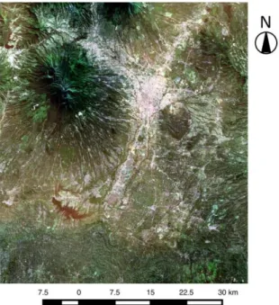
Fig. 1. Study site in Malang Regency, East Java-Indonesia
Fig. 2. A Landsat8-OLI image of the study area. The multi-band data was shown with the true color image.
Fig. 3. Relative frequency of the land-cover types in ground truth data for each class distinguished by the unsupervised classification of the satellite image.
Fig. 4. Land-cover map derived by the analyses of the Landsat8-OLI/TIRS image.
Fig. 5. Proportion of area of the five land-cover types in the study area.
Fig. 6. Spatial distribution of landscape diversity index (H’) calculated based on the relative dominance of different combinations of land-cover types.
Fig. 7. Spatial distribution of the potential hotspots (white) detected as the upper 5 percentile of H’ calculated based on the relative dominance of different combinations of land-cover types
Fig. 8. Relationship between H’ and environmental factors.
Fig. 9. Location of the study site.
Fig.10. Spatial arrangement of agroforestry (AF) patches and quadrats for plant survey
Fig. 11. A schematic illustration of distinguishing “interior-common species” and
“edge-common species”
Fig. 12. Number of plant species found in each agroforestry (AF) type. Figures in parentheses are the number of native species.
Fig. 13. Proportion of numbers of species (all species (A) and native species (B)) with reference to different original habitats.
Fig. 14. Comparisons of the composition of the interior- and edge-common species for P-T (A) and P-E (B) with reference to original species habitats
Fig. 15. Species area curves drawn for the interior- and the edge-common species for P-T (A-1 and A-2) and P-E (B-1 and B-2).
Fig. 16. Comparisons of the sky factor measured at the edge and the patch interior along two combinations of different agroforestry types: P-T (A) and P-E (B).
Fig. 17. Comparisons of the soil water content (SWC) measured at the edge and the patch interior along two combinations of different agroforestry types: P-T (A) and P-E (B).
Fig. 18. Comparisons of the ground cover by litter and vegetation at the edge and the patch interior along two combinations of different agroforestry types: P-T (A) and P-E (B)
Fig. 19. Examples of stand floor cover in P (A), T (B), and E (C).
11 11 16
18 19 21 22
23 29 30 32 36 36 38 39 40
41 41 42
Table contents
Table. 1. Land-cover types used in the five methods of H’ calculation
Table. 2. Stand structure and growing crops of the studied three agroforestry (AF) patches
Table. 3. Characteristics and occurrence of plant species found in the study site
14 30 35
1 Abstract
Asian tropics including Indonesia is one of the most serious regions suffering from the decline of biodiversity due to the deforestation and forest degradation. As countermeasures to prevent further degradation of biodiversity, several international plans have been launched. REDD+
(Reducing Emissions from Deforestation and forest Degradation in developing countries) is one of those schemes, and is expected to prevent the spread of deforestation in tropical regions. However, as REDD+ evaluates enhancements in forest carbon sequestration, there is serious concern that it will promote extensive monoculture of fast-growing species which causes further losses of biodiversity. Therefore, other effective strategies of land use for conserving biodiversity are strongly desired as a safeguard against this potentially negative aspect of REDD+. This study aimed to provide effective measures for REDD+ safeguard from the context of landscape and plant ecology focusing on agriculture-forest mixed landscapes and agroforestry systems.
Firstly, land-cover complexity of the agriculture-forest mixed landscapes were analyzed with different datasets of land-cover types to explore the optimal method for setting the potential biodiversity hot spots as the conservation targets at a regional scale. A land-cover map of a sample area in East Java was generated to have five major land-cover types (forest, agricultural land, bare land, water, and residential) by the unsupervised classification of a Landsat8-OLI image. Based on the land-cover map,
2
Shannon’s diversity index (H’) was calculated for each cell using moving window of 11 x 11 pixels (10.98 ha) throughout the study area by five calculation methods with different combinations of land-cover types. Then, the cells of the upper 5% in H’ was selected as the potential hotspots in terms of highly complex patch mosaics. The detected potential hotspots were compared referring to the criteria of usefulness; e.g., aggregated distribution patterns or less sensitiveness to the residential patches. The results demonstrated that the dataset of four land-cover types (forest, agriculture, water and bare land) was thought to be most suitable to detect the conservation targets at a regional scale.
Secondly, plant species diversity in the in the understories of three agroforestry (AF) patches dominated by pine (Pinus merkusii), teak (Tectona grandis) and eucalypt (Eucalyptus camaldulensis) in East Java was investigated in order to evaluate the potential conservation value of AF mosaics against extensive monocultures. The results indicated that the variability among different AF types contributed to more than half of the total and native species richness in the studied AF patches, suggesting an advantage of the having landscape consist of mosaics of different AF types for the conservation of plant species diversity. However, the results also indicated the limited edge effects in terms of promoting the coexistence of plants with different characteristics within a patch, compared to typical forest edges such as those between closed forests and open grasslands.
These findings are thought to be useful in developing REDD+ safeguard by setting the target landscape for conservation at a regional scale, and by
3
providing desirable landscape design to reduce the negative impacts of monocultures.
4 Chapter 1. Introduction
1.1. Background: Needs of feasible and effective safeguards for REDD+
Environmental issue has received much attention in recent years due to its degradation of biodiversity, which offer important for ecosystem services. Maintenance and restoration of ecosystem services are essential for sustainable community welfare, and biodiversity is the essential element supporting various kinds of ecosystem services (United Nations, 2005).
However, biodiversity has been deteriorated during the last century all over the world mainly due to overuse of ecosystems represented by deforestation and unfettered monoculture production expansion (Jepma 1995; Bawa &
Dayanandan 1997), resulting in severe degradation of ecosystem services (Putz et al. 2001; Gibson et al. 2011). Indonesian forest has an important role in Southeast Asia and even the world, because of that extensive deforestation in Indonesia is a cause for global concern as it contributes substantially to land-based global carbon emissions. Global Green House Gas (GHG) emissions accounted for nearly 20% of deforestation and degradation (Cadman. 2017).
Reduction Emission Deforestation and Forest degradation (REDD+) is expected to prevent the spread of deforestation in tropical regions. Currently, REDD+ conserving and enhancing forest carbon stocks, and sustainably managing a forest have become a reference framework for national forest governance across many tropical and sub-tropical forest countries. As
5
countermeasures to prevent further degradation of biodiversity, several international plans have been launched after the Millennium Ecosystem Assessment conducted by the United Nations (Millennium Ecosystem Assessment 2003, 2005). REDD+ (Reducing Emissions from Deforestation and forest Degradation in developing countries) is one of those schemes (Lund et al. 2017), and is expected to prevent the spread of deforestation in tropical regions. However, as REDD+ evaluates enhancements in forest carbon sequestration, there is serious concern that it will promote extensive monoculture plantation of fast- growing species, which causes further losses of biodiversity. Monoculture plantation causes degradation of biodiversity and ecosystem services because it attaches importance to timber production and forest carbon sequestration. For example, production of agro-fuels from palm oil and soy-based cattle food have often been achieved by conversion of forests ecosystems to non-forest uses (Puppim de Oliveira et al., 2013).
Therefore, effective strategies of land use for conserving biodiversity are strongly desired as a safeguard against this potentially negative aspect of REDD+.
Safeguards have been identified as an important element to ensure the effective implementation of REDD+, including conservation, sustainable management of forests and enhancement of forest carbon stocks, in developing countries and to avoid, or at least minimize, negative governance, social, and environmental impacts. Nevertheless, most of the currently proposed safeguards are of effort goals set for county scale, and there are still
6
less concrete and effective studies and established methods that can be applied for regional-scale management.
1.2. Approaches detecting hot spots from landscape context
Hot spot is an area that has high biodiversity and also has an important role in safeguard of biodiversity, preserving endangered species and providing ecosystem services, such as water filtration or air cleaning. The term "hotspot" often refers to areas where high amounts of diversity on ecosystem services are available (Arnold & Lutzoni, 2007; Cimon-Morin, Darveau, & Poulin, 2013; Goreno, Romaine, Mittermeier, & Walker- Painemilla, 2012), is one of the useful ideas for the strategy to set the conservation targets within a region.
In particular for REDD+ safeguards, the hotspots should consider not only the primary ecosystems such as old growth natural forests but also the secondary natures in traditional farming or forestry landscapes, because the pressure of extensive monoculture could target these landscapes (Edwards et al., 2010).
The hotspots should basically be designated with assessment of diversity at species level. However, setting hotspots of secondary nature with species-level assessment at a regional scale might be quite difficult. As a substitute to the assessment at species level, land-cover types, which can be easily analyzed at broad scale based on geographic information, is the useful measure to identify the potential hotspots at landscape level, as land-cover
7
changes are key drivers of the loss of biodiversity and ecosystem services (Schröter et al., 2005). In addition, habitat heterogeneity in terms of different land-cover types plays an important role in regulating the distribution of species (Benton, Vickery, & Wilson, 2003; Billeter et al., 2008; Harms, Condit, Hubbell, & Foster, 2001; Tews et al., 2004). Thus, patch mosaic landscapes consisting of different land-cover types could be conservation targets as the potential biodiversity hotspots that encompass higher biodiversity compared to extensive monoculture landscapes.
According to Scharsich et al. (2017), to decide whether the state of protection or management of surrounding areas have a quantifiable effect on land use and land cover, remote sensing provides a valuable data source.
Particularly in order to observe large, heterogeneous or poorly accessible regions, remote sensing data are a good choice.
Satellite images constitute the main tool to infer land use and land cover, all over the world and are used to detect changes and developments in various landscapes. Today, a broad range of satellite images and other remote sensing data are freely available and some data even date back to the middle of the last century. Therefore, it is possible to monitor and analyze the development of almost any region in the world and safeguard areas like hotspot with satellite images and remote sensing, the aim is to protect biodiversity.
8
1.3. Proposing alternatives to extensive monocultures
In order to make the safeguards feasible and effective in the actual management of agriculture-forest landscapes, alternatives to the extensive monoculture considering the function of patch-mosaic landscape are strongly desired to be proposed. Agroforestry (AF) is a potential means to conserve biodiversity while continuing agricultural and forestry production (Wicaksono et al. 2011). Monocultures of fast-growing tree species often form densely closed canopies that eliminate most plant species and reduce diversity of the understory by heavy shade (Bekessy & Wintle 2008). In contrast, AF, which grows agricultural crops beneath the canopy of planted trees, could provide more favorable microenvironments for the growth of many plants compared to monocultures. Furthermore, different types of AF with different tree species can support plants of different life-history traits by forming different understory environments (Montagnini et al. 2004). Thus, mosaic landscape consisting of different types of AF may have great advantages over the extensive monocultures in terms of biodiversity conservation by 1) supporting higher species diversity at the landscape scale, and 2) forming within-patch heterogeneity due to edge effects (Jose. 2009) between different patches. To study the advantages of AF mosaics, plant species occurrence should be assessed with reference to the types of AF and their adjacency. However, this kind of information is still quite limited.
9 1.4. Objective of this study
This study aimed to provide effective measures for REDD+ safeguard from the context of landscape and plant ecology focusing on agriculture-forest mixed landscapes and agroforestry systems.
In the Chapter 2, land-cover complexity of the agriculture-forest mixed landscapes in East Java, Indonesia were analyzed with different datasets of land-cover types to explore the optimal method for setting the potential biodiversity hot spots as the conservation targets at a regional scale.
In the Chapter 3, the occurrence of plant species in the understories of typical AF types were investigated in East Java, Indonesia as a case study to evaluate the potential conservation value of AF mosaics against extensive monocultures.
10 Chapter 2.
Detecting potential biodiversity hotspots for development of REDD+
safeguards based on analyses of land-cover complexity in East Java, Indonesia
2.1. Objectives
I aimed to examine a new method to detect the potential biodiversity hotspots in terms of complex patch mosaics of various land-cover types as the conservation targets at a regional scale in East Java, Indonesia. The specific objectives of this study were 1) to suggest the optimal combinations of land- cover types to detect the potential hotspots by applying Shannon’s diversity (H’) index for land-cover diversity, and 2) to examine the effects of environmental factors on the distribution of potential hotspots to discuss the major drivers of forming the potential hotspots.
2.2. Methods
2.2.1. Study area
The study was conducted in Malang, East Java (Fig. 1). Geographically this region lies between 7° 59' 2.0688'' S and 112° 37' 17.0076'' E, and also has elevation from 473 to 3,300 m a.s.l. Malang is one of the most forested areas in East Java. Malang Regency is located between two groups of mountains;
11
Mount Semeru the highest mountain on Java, and Bromo-Tengger-Semeru national park to the east. The study area is approximately 3,052 km2 and is comprised of numerous agricultural lands, agroforestry, and small forest fragments with a wide variety of forest types, including lowland, mountain and seasonal forests.
Fig. 1. Study site in Malang Regency, East Java-Indonesia.
Fig. 2. A Landsat8-OLI image of the study area. The multi-band data was shown with the true color image.
12 2.2.2. Data source
A satellite image (Fig. 2) acquired by Landsat8-OLI/TIRS (path 118, row 66) on 16 June 2014 (in a rainy season) was used to interpret land-cover conditions. This image was selected from twelve images of the same region to have less than 10% cloud cover for minimal cloud contamination. The selected image was geo-referenced according to the UTM coordinate on a geographical information system (Quantum GIS). The dataset includes the metadata file and following Landsat 8 band (16 bit raster).
2.2.3. Classification of land-cover types
The unsupervised classification method was used to classify the land- cover types. Unsupervised classification does not require human to have the foreknowledge of the classes, and mainly using clustering algorithm to classify an image data. After clustering pixels of the Landsat image by unsupervised procedure by using a function in GIS (Semi-Automatic Classification Plugin), obtained classes were re-categorized into five main categories which might have effects on the formation of the potential hotspots (forest, agricultural land, bare land, water and residential area) by comparing actual land use (the ground truth) of randomly selected 241 sample points.
For the ground truth data, I used Google Earth and ground photographs taken in 2015 to identify the corresponding land-cover types in each class to improve the accuracy of the classifications, because no official reference data
13
on the actual land use or land cover was available for the study area. The use of Google Earth to derive reference data has been suggested in many previous studies (e.g. Scharsich et al., 2017; gong et al., 2013).
2.2.4. Analyses of land-cover diversity
For evaluation of land-cover diversity, Shannon’s diversity index (H’) was used for each cell using moving window of 11 x 11 pixels (10.98 ha) in the whole study area excluding pixels of outermost 5 rows and columns. H’ was calculated by the following equation;
H’ =-Σpi ln pi
Where, pi is the relative dominance of i th land-cover types within a given landscape. In order to detect the different effects of land-cover compositions on the evaluation of potential hotspots, H’ was calculated for five methods using various combinations of land cover types (Table 1): method a) all five land cover types, method b) four land-cover types excluding residential, method c) forest, agriculture and bare land, method d) forest, agriculture and water, and method e) forest and agriculture. All the calculations were based on the dominance to all five land-cover types, that is, method b) - e) indicate partial values for the adopted land-cover types of the total H’ of five land- cover types.
14
Table 1. Land-cover types used in the five methods of H’ calculation.
Methods Land-cover types
Method-a forest, agriculture, water, bare land, residential Method-b forest, agriculture, water, bare land
Method-c forest, agriculture, bare land Method-d forest, agriculture, water Method-e forest, agriculture
After each calculation of H’, the cells of upper 5 % in H’ was adopted as the potential hotspots in terms of highly complex patch mosaics of land-cover types. The distribution of the hotspots detected by the five calculation methods were compared each other in order to evaluate their appropriateness with reference to the following criteria which consider the requirements for setting effective conservation targets at a regional scale: Criterion A): to exclude properly the large cities and extensive monoculture landscapes, Criterion B): to exclude properly the patch mosaics affected residential patches, which will not encompass high biodiversity, Criterion C): to show the contagious (aggregated) distribution of hotspots with a certain extent for set ting the important area at a regional scale and, Criterion D): to detect the universal hotspots without strong biases to specific a land use.
To examine the effects of environmental factors on the distribution of the potential hotspots, relationships between the H’ values to elevation, slope inclination and the urbanization index were analyzed. Elevation and slopes for each pixel were obtained from a digital elevation model supplied from USGS. The urbanization index was calculated as the average of the
15
population of 7 cities within the study area (see Fig. 4) divided by distance from the given pixel to the city. Thus, the larger value of this index means higher degree of urbanization. These factors were divided into four 25 % quantiles of the number of pixels according to their values from small (class 1) to large (class 4). Then, the H’ was compared between the classes for each environmental factor.
2.3. Results
2.3.1 Classification and distribution of land-cover types
15 classes were distinguished by the unsupervised classification of the satellite image. By comparing with the sample points of ground truth data, these 15 classes were recategorized into 5 categories according to the relative frequency of actual land-cover types (Fig. 3).
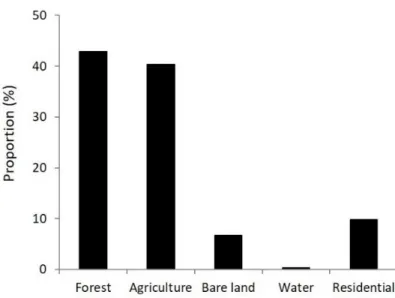
Fig. 4 shows the land-cover map the five categories. Forest is the most dominant category of land cover occupying 43 % of the study area (Fig. 5), followed by agricultural land (40 %). Bare land and residential area counted 7 and 10 % of the study area, respectively. Water occupied the smallest area (0.3%).
16
Fig. 3. Relative frequency of the land-cover types in ground truth data for each class distinguished by the unsupervised classification of the satellite image. Fifteen classes by satellite image analyses were recategorized into five categories according to the dominant land- cover types.
As the features of spatial distribution of land-cover types (Fig. 4), a large residential area (A in Fig. 4) was found around Malang City, which is the capital with the highest population density and lowest forest availability in the study area. Most of the other residential areas were aligned along the main national roads (black lines in Fig. 4). The mosaics with small residential patches were also found the area surrounding the main national roads.
A distinctly extensive area of agricultural land was detected in the southern-central part of the study area (B) near Gondang legi City. Other major agricultural lands were distributed relatively close to the main roads.
In contrast, major forest covers were found to be situated distant from the main roads, around Mt Kawi in north-western part (C) and in southern part
17
of the study area (D). On the lower slopes of Mt Kawi, strip-shaped patches were found along the topography: forest patches along gullies, and agricultural or bare land patches on gentle ridges (Fig.2 and Fig.4). However, middle slopes were mainly covered by large forest patches. In contrast, in the eastern part of the study area (E), agricultural land was codominant with forest even distant from the main roads. In this area, which is a part of the slope of Mt Bromo located in outside (east) of the study area, a lot of residential patches were scattered.
Bare land patches were also found in and around agricultural patches relatively close to the main road and cities. Water cover was mainly found in and around a dam lake located in south-western part of the study site.
18
Fig. 4. Land-cover map derived by the analyses of the Landsat8-OLI/TIRS image. Five land-cover types were shown by different colors of 30 m x 30 m pixels. Meanings of alphabets in the figure are explained in the text.
19
Fig. 5. Proportion of area of the five land-cover types in the study area.
2.3.2 Distribution of the potential hotspots obtained by different methods
The spatial distribution of land-cover diversity index (H’) and the potential hotspots obtained by the different combinations of land-cover types were shown in Fig. 6 and Fig. 7, respectively The H’ around Malang City is commonly low throughout the different methods, i.e., different combinations of land-cover types (A in Fig. 6). Consequently, the hotspots detected by the all methods uniformly excluded the Malang City (A Fig. 7). Similarly, the area dominated by single land-cover type (agriculture) showed equally low H’
(B in Fig. 6), and was excluded from the potential hotspots by every method (B in Fig7). In the calculation method a) adopting five land-cover types (Fig.
6a), the landscapes including small patches of residential area around Malang City (F1 and F2) or Mt Kawi along the road (F3 and F4) showed high
20
H’ (Fig. 6), probably reflecting small patches of residential area (Fig. 4 and 6f).
These high H’s resulted in evaluation of many potential hotspots outside of the Malang City affected by small patches of residential area (Fig. 7a). The calculation method b) without using residential areas showed slightly different distribution of H’ (Fig. 6b) compared to the method a) (Fig. 6a). The potential hotspots were not detected around the large city or the main roads (F1, F2, F3 and F4 in Fig. 7b). Instead, several potential hotspots were additionally detected at the boundary of agriculture and forest dominated areas in the southern part (G1 and G2 in Fig.7b).
The distribution H’ calculated by method c) which adopted forest, agriculture and bare land, was similar to those by the method b). The method c) added only few and small potential hotspots at the north of the dam lake (H in Fig. 7c), where many small bare land patches were distributed.
The method d) and e) generated lower contrast of H’ compared to the former three methods (Fig. 6d and 6e), resulting in widely scattered, small and many potential hotspots (Fig. 7d and 7e). In the methods d) which adopted forest, agricultural land and water, relatively large potential hotspots were detected at lake shore (I in Fig. 7d). However, these potential hotspots were not found by the method 3) which used only forest and agricultural land cover (Fig. 7e)
21
Fig. 6. Spatial distribution of landscape diversity index (H’) calculated based on the relative dominance of different combinations of land-cover types: a) all five types, b) agriculture, forest, bare land, and water, c) agriculture, forest and bare land, d) agriculture, forest and water, e) forest and agriculture. Panel f) was the land-cover map (same as Fig.
4) shown as a reference for comparisons. Meanings of alphabets in the figure are explained in the text.
22
Fig. 7. Spatial distribution of the potential hotspots (white) detected as the upper 5 percentile of H’ calculated based on the relative dominance of different combinations of land-cover types: a) all five types, b) forest, agriculture, bare land and water, c) agriculture, forest and bare land, d) agriculture, forest and water, e) forest and agriculture. Panel f) was the land-cover map (same as Fig. 4) shown as a reference for comparisons. Meanings of alphabets in the figure are explained in the text.
23 2.3.3 Environmental factors
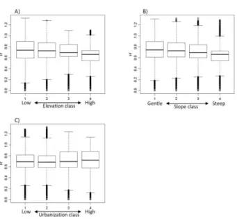
In this study, clear responses of H’ to the environmental factors were not observed (Figs. 8).
Fig. 8. Relationship between H’ and environmental factors i.e. A) elevation, B) slope inclination, C) urbanization index. H’ was calculated by the Method b) adopting four land-cover types. See the text for details.
Classes of environmental factors in x-axes were divided into 25 % quantiles of the number of pixels according to their values from small (class 1) to large (class 4).
24 2.4. Discussion
2.4.1. Optimal method for detecting the potential hotspots
Evaluating diversity of landscape structure is the basis for understanding landscape scale biodiversity and diversity in plant communities. Among the 5 potential hotspots, the calculation of H’ with four land-cover types (forest, agriculture, water and bare land) was thought to be most suitable to set conservation targets at a regional scale, because the potential hotspots by this method showed aggregated distribution patterns, and was less sensitive to the small residential patches.
The spatial distribution of the potential hotspots detected in this study indicated that the large city and extensive agricultural fields, which may have low biodiversity, was well expressed by H’s of the all methods (Fig. 6 and Fig. 7), suggesting the all methods texted here fulfill the Criterion A.
However, the result of the method a) adopting five land-cover types suggested the possible errors of this method, such as detecting inappropriate hotspots affected by small residential patches (Fig. 6a). Thus, this method was evaluated unsuitable with reference to the Criterion B. The method b) which excluded residential land cover from its calculation indicated that this method is thought to be better than method a), because H’ was less sensitive to the small residential patches in spite of its ability to detect low H’ of the large city and extensive farmlands. The method c), which adopted bare land with forest and agricultural land, may be applicable to the study area
25
because this method produced the similar result as method b), though it was slightly sensitive to a single land cover type.
The methods d) and e) would not be suitable to set sizable conservation target areas referring to the Criterion 3, because the potential hotspots in these two methods were relatively scattered compared to the other three maps, indicating an unsuitable feature for detecting the hotspots which should be aggregated in parts of the region.
The results of methods c) and d) suggested that adopting one of bare land or water in the calculation of H’ will give contrasting results in detecting hotspots of specific targets. Bare land would be useful if the frequent disturbances, which make bare land, are important for setting conservation targets as the driver of biodiversity. On the other hand, for the case where aquatic or riparian ecosystem should be taken into account in detecting hotspots, water would be the key land-cover type. Thus, these two methods are thought to be useful when the specific conservation target is clear.
However, the too strong bias to a specific land-cover type due to single use of these tow types may not suitable for setting conservation area for a universal, broad range of biodiversity, referring to the Criterion 4. Thus, the landscape planners and managers should be carefully deal these land-cover types in the calculation of H’ as the indicator of hotspots.
In conclusion, the method b) can be proposed to be the most optimal method to detect the potential biodiversity hotspots based on the landscape analysis, because this method was not too sensitive to a single land-cover
26
type, and provides relatively universal hotspots for biodiversity with their contagious distribution for setting conservation targets.
2.4.2. Possible drivers of the potential hotspots
In this study, clear responses of H’ to the environmental factors were not observed (Figs. 8). This might be partly due to the large fluctuation of H’.
However, slight tendencies of H’ to decrease at high elevation or steep slopes (Fig.7a and 7b) might be affected by the high dominance of forest patches in mountainous area where agricultural land use is difficult.
I expected the effect of urbanization on the distribution of potential hotspots, because urbanization would promote intensive agriculture with extensive monocultures around urban areas. According to this hypothesis, combined with the extensive forest in mountainous area, the potential hotspots could distribute between urban and remote areas. The landscape structure (Fig. 4) and the potential hotspots (Fig. 7) partly demonstrated these features. However, the hypothesis was not numerically supported in this study by the urbanization index taking into account the major cities (Fig.
8c). This may be owing to the five patch mosaics of forest and agricultural land in eastern part of the study area (E in Fig 4), which had contrasting landscape structure to the western and southern part (C and D in Fig. 4), in spite of similarly remote situation from the cities and the main roads.
Therefore, further parameterization using more detailed or broad factors will
27
be needed to explain the effects of the natural and social environment on the land cover diversity at a regional scale.
28 Chapter 3.
Occurrence of plant species in three types of agroforestry patches neighboring each other in East Java, Indonesia
3.1. Objectives
I aimed to examine the advantages of AF mosaics. For this purpose, I investigated plant species diversity in the understories of three agroforestry (AF) patches dominated by pine (Pinus merkusii), teak (Tectona grandis) and eucalypt (Eucalyptus camaldulensis) in East Java in order observe the traits of plant occurrences in relation to the AF types and their adjacency. Based on the results, I discussed the differences in species occurrence among AF types and effects of adjacent AF.
3.2. Methods
3.2.1. Study site
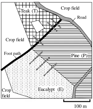
The field survey was conducted in AF sites near Malang City, East Java, Indonesia (Fig. 9), consisting of three patches of common AFs in a region dominated by different planted tree species; pine (Pinus merkusii: Merkus pine), teak (Tectona grandis: common teak) and eucalypt (Eucalyptus camaldulensis: river red gum) (hereafter, abbreviated as P, T, and E,
29
respectively). The study site was situated on a gentle mountain slope (slope inclination < 5°) at 890-950 m above sea level. The patch of P was adjacent to T and E (Fig. 10). Stand structure of the three AF patches are summarized in Table 2. I could not determine the previous land use of the study site before developing the current AFs.
Fig. 9. Location of the study site.
Study site Java
Sumatera
Kalimantan
100E 110E
0
10S
30
Fig.10. Spatial arrangement of agroforestry (AF) patches and quadrats for plant survey. Grey lines and open circles denote transects and quadrats, respectively.
Table 2. Stand structure and growing crops of the studied three agroforestry (AF) patches.
AF type
Tree density
(/ha)
DBH *1 (cm)
Height *1 (m)
Crop species
Pine (P) 667 20.3 (5.0-30.0) 12.6 (4.0- 18.0)
Napier grass *2, Banana Teak (T) 750 14.0 (10.0-
25.3) 9.2 (8.5- 10.0)
Coffee, Cassava
Eucalypt
(E) 400 10.2 (4.3-21.3) 7.6 (3.3- 16.5)
Napier grass, Cassava
*1 DBH and Height are shown by average (min-max) values.
*2 Napier grass (Pennisetum purpureum) are harvested every month and used for cattle.
Crop field
Crop field
Crop field Teak (T)
Pine (P)
Eucalypt (E)
Road
Foot path
100 m
31 3.2.2. Field survey
I placed three transects across the border of P-T and P-E, respectively (altogether 6 transects), and established sample quadrats sized 1 m × 1 m with different distance from the patch border: P at 10 and 20 m; T at 5, 10, 20 and 30 m; and E at 5, 10, 20, 30 and 50 m from the patch border, respectively (Fig. 10). Consequently, the number of quadrats placed in P, T and E were 12, 12 and 15, respectively. The quadrats in P and T were placed with different number and location from those in E in order to avoid the effects of edges facing the patches out of the target. All vascular plants (height < 1 m) occurring in the quadrats were recorded with their species name. At each quadrat, I measured conditions of the stand floor. Visual cover of the ground surface by litter (leaves of planted trees and others) and vegetation were measured. Hemispherical photographs were taken at 1 m above the ground surface using a fish-eye lens (FC-E9, Nikon), and soil water content (SWC) was measured using a TDR sensor (Hydrosense, Campbell) with 12cm probes.
Field surveys were carried out in September (at the beginning of the rainy season, and in the fallow period) in 2016, 2017 and 2019 separately for different transects but for all patches.
32
Fig. 11. A schematic illustration of distinguishing “interior-common species”
and “edge-common species”. “Edge” was defined as those within 10 m from the patch border, and others were defined as “patch interior”.
Common species occurring in the interiors of both patches (shown by grey bars) were designated as “interior-common species” irrespective of their presence/absence in the edge. Those that were not found in one of the interiors (shown by white bars) were designated as “edge- common species”.
3.2.3. Data analyses
Plant species found in the quadrats were grouped according to their original habitats into 6 groups: woodland, forest edge, grassland, wetland, generalist species, and others (unknown) based on descriptions in the literatures (Lundholm & Marlin 2006). Species for which the original habitat is not described in the literature were considered as “others”. Native species were also distinguished from naturalized species. By pooling three transects for each AF type, I counted the number of species specific to each AF type
10m 0m 10m
Edge-common species Interior-common species
Edge Patch interior
Patch interior
Patch border
33
(those occurring in only one type), and species common to different types (i.e., P-T common, P-E common, T-E common, and P-T-E common species), and compared them with reference to the species groups. The same analyses were performed for native species. Further, by assuming that the quadrats placed at 10 m from the patch border represent “edges” and others “patch interiors”, I classified the species common to P-T and P-E into 1) interior-common species (I-common) which occurred in the interiors of both patches irrespective of their presence/absence at the edge, and 2) edge-common species (E-common) which occurred in the edges and were not found in one or both of the interiors (Fig. 11). Species-area curves of I-common and E- common species were drawn for all and native species separately by using PC-ORDTM 7, a based software for vegetation analyses. I calculated the sky factor (SF, the ratio of open canopy) from the hemispherical photographs. I compared SF and SWC between the edges and interiors for P-T and P-E combinations (Steel-Dwass test).
3.3. Result
3.3.1. Total and specific species of each AF type
Altogether 52 species were recorded in the three AF types; more than half of them were native species (29 spp.: 56%) (Table 3). P, T and E consisted of 32, 20, and 35 species including 16, 11 and 18 native species, respectively, indicating lower richness of all and native species in T compared with P and
34
E (Fig. 12). There was no clear difference in the proportion of native species among AF types. P, T and E had 8, 6 and 13 species that were specific to each type, including 4, 5 and 7 native species, respectively (Fig. 10). These specific species (altogether 27 spp.; 16 spp. among them were native species) occupied more than half of the total and native species found in this study. The species specific to E were characterized with a high proportion of grassland species (4 spp.: 30%) compared to P and T in which only one grassland species was found (Fig. 11(A)). A similar trend was observed for native species; 2 out of 7 species in E were grassland species (Fig. 11(B)). In contrast, the specific species of T, contained only 6 species (consisting of 5 native species) with no wetland species, and showed a larger proportion of woodland and edge species (altogether half of 6 spp.; but 2 out of 5 spp. for native species). P had intermediate characteristics with 1 or 2 plants for each various habitat type.
35
Table 3. Characteristics and occurrence of plant species found in the study site.
Species Original
habitat
Native/
Naturalized
Occurrences in each AF type
T P E
Acalypha australis edge Naturalized + + +
Adiantum diaphanum others Native +
Ageratum conyzoides generalist Naturalized + + +
Artemisia vulgaris wetland Native +
Atryrium ascendens others Native +
Borreria alata woodland Native + +
Brachiaria decumbens grassland Native + +
Calopogonium mucunoides grassland Native +
Cardiospermum halicacabum others Native +
Centella asiatica wetland Native + +
Centrosema pubescens grassland Naturalized + + +
Chamaesyce hirta others Naturalized +
Chromolaena odorata generalist Naturalized +
Citrus sinensia woodland Naturalized +
Coleus amboinicus edge Naturalized +
Commelina diffusa generalist Naturalized + + +
Conyza sumatrensis grassland Naturalized + +
Cynodon dactylon grassland Naturalized +
Cyperus kyllingia grassland Native +
Cyperus rotundus wetland Native +
Diplazium esculentum others Native + +
Diplazium stuebelianum wetland Native + +
Elephantopus scaber edge Native +
Emilia sonchifolia generalist Native + +
Eragrostis curvula grassland Naturalized +
Eragrostis tenella grassland Native +
Eupatorium inulifolium woodland Native + + +
Ficus septica woodland Native +
Imperata cylindrica grassland Native + +
Ipomoea triloba edge Naturalized +
Leersia hexandra grassland Native +
Lespedeza stipulacea others Native + + +
Leucaena leucocephala edge Naturalized +
Lindernia crustancea wetland Naturalized +
Manihot esculenta generalist Native +
Mecardonia procumbens others Native +
Mimosa pudica woodland Native +
Oplismenus undulatifolius edge Native + + +
Oxalis corniculata others Native + +
Oxalis latifolia generalist Naturalized + + +
Paspalum conjugatum others Naturalized + +
Pennisetum purpureum grassland Naturalized + +
Phyllanthus lepidocarpus others Naturalized + +
Pityrogramma calomelanos others Native + +
Polygonum hydropiper wetland Naturalized +
Pseudelephantopus spicatus edge Native + +
Pteridium aquilinum edge Native +
Setaria sphacelata grassland Naturalized + +
Sida rhombifolia generalist Native +
Stachytarpheta jamaicensis generalist Naturalized + + +
Synedrella nodiflora edge Naturalized + + +
Tridax procumbens others Naturalized +
1
36
Fig. 12. Number of plant species found in each agroforestry (AF) type.
Figures in parentheses are the number of native species.
Fig. 13. Proportion of numbers of species (all species (A) and native species (B)) with reference to different original habitats. Figures in parentheses are the total number of species in each category.
10 (3) 3 (2)
11 (7) 1 (1)
8 (4) 6 (5)
13 (7)
Pine (P): 32 (16) Teak (T): 20 (11)
Eucalypt (E): 35(18)
P-T:
13 common / 39 total =33% (all spp.) 5 common / 22 total =23% (native spp.)
P-E:
21 common / 46 total =46% (all spp.) 10 common / 24 total =42% (native spp.)
T-E:
11 common / 44 total =25% (all spp.) 4 common / 25 total =16% (native spp.)
100
0.00.20.40.60.81.0
80
60
40
20
0
T P E P-T P-E T-E P-T-E
Species specific to each type
Species common to different type
Proportion of species number (%)
(5) (4) (7) (5) (10) (4) (3) (B) Native species
0.00.20.40.60.81.0
100
80
60
40
20
0
T P E P-T P-E T-E P-T-E
Species specific to each type
Species common to different type
Proportion of species number (%)
(6) (8) (13) (13) (21) (11) (10) (A) All species
others generalist wetland grassland edge woodland
37 3.3.2. Common species to different AF types
Ten species were found in all AF types (P-T-E), accounting for 19% of the total 52 species (Fig. 12), with a large proportion of generalists and forest edge species (4+4 spp.: 80%) (Fig. 13(A)). Among them, however, only 3 species (including one woodland and one edge species) were native species (Fig. 12, Fig. 13(B)). The numbers of the all species common to P-T, P-E, and T-E were 13, 21, and 11, which occupied 33%, 46%, and 25% of the pooled species of each combination (39, 46, and 44), respectively (Fig. 12). The species common to P-E were much greater in number than those of P-T and T-E, and had a large proportion of grassland species (6 out of 21 spp.: 29%) (Fig. 11(A)). This trend was also true for native species; number of native species common to P-E (10) were much greater than those of P-T (5) and T-E (4), and consisted of 2 grassland species while P-T and T-E had no grassland species (Fig. 11(B)). In contrast, P-T and T-E had a higher proportion of generalists (4 spp.: 31% and 36%, respectively) (Fig. 13(A)), but these generalists were non-native (naturalized) species. Consequently, native species common to P-T and T-E included no generalist (Fig. 13(B)).
In P-T transects, 6 I-common and 4 E-common species were found, including 1 woodland species and 2 forest edge species in the I-common species (Fig. 14(A)). I-common species increased up to ca. 5 m2 of increased sample area, while the number of E-common species became stable above 3 m2 of sample area (Fig. 15(A-1)). Regarding native species, only 2 species
38
were found for each of I common and E-common species (Fig. 14(A)), demonstrating similar increase of the number of species along the sample area (Fig. 15(A-2)). In P-E transects, 11 I-common species consisting of various habitat types were found, while the number of E-common species was 4, the same as in P-T transects (but 2 forest edge species and 2 grassland species) (Fig. 14(B)). Increases in the number of I-common and E-common species along the increase of sample area were observed up to ca. 10 m2 and 3 m2, respectively (Fig. 15(B-1)). The trend for E-common species was almost the same as that for P-T transects. Regarding native species, I-common had similar trends as those found in all species in terms of various habitat types (Fig. 14(B)) and the species number increasing up to 10 m2 (Fig. 15(B-2)), while the number of species was 6. In contrast, native E-common included only one edge species.
Fig. 14. Comparisons of the composition of the interior- and edge-common species for P-T (A) and P-E (B) with reference to original species
10 8 6 4 2 0 12
10 8 6 4 2 0 12
Interior- common
Edge- common
Number of species
Interior- common
Edge- common Interior-
common Edge- common
All species Native species Interior-
common Edge- common All species Native species
(A) P-T common (B) P-E common
P-interior: 3m² T-interior: 9m² Edge: 9m²
P-interior: 3m² E-interior: 12m² Edge 9m²
Number of species
others generalist wetland grassland edge woodland
39
habitats. Total quadrat area used for counting species are shown at the top of the bars.
Fig. 15. Species area curves drawn for the interior- and the edge-common species for P-T (A-1 and A-2) and P-E (B-1 and B-2). Solid and dotted lines indicate the average and min-max ranges, respectively.
3.3.3. Physical environments and ground cover
The SF showed no significant difference among patch interiors and edge within and between P and T (Fig. 16A)). There was also no significant difference in P-E, though the SF tended to increase from the interior of P
Edge-common spp.
Interior-common spp.
Interior-common spp.
Edge-common spp.
0 5 10 15
15
10
5
0
0 5 10 15
15
10
5
0
(A-1) P-T common (all species)
(B-1) P-E common (all species)
Number of species
Number of quadrats (1m²)
Number of species
Number of quadrats (1m²)
0 5 10 15
0 5 10 15
0 1 2 3 4 5 6 7
Number of species
Number of quadrats (1m²)
Number of species
Number of quadrats (1m²) Interior-common spp.
Edge-common spp.
Interior-common spp.
Edge-common spp.
(A-2) P-T common (native species)
(B-2) P-E common (native species)
0 1 2 3 4 5 6 7
Min-max range Average
40
(15.0%) to the interior of E (26.2%) across the edges (Fig. 16(B)). Soil moisture content tended to decrease from the interior of P (12.8%) to the interior of T (9%); however, the difference was not significant (Fig. 17(A)). P-E showed almost the same values of soil moisture content throughout the edge and the interior of both patches (Fig. 17(B)). Ground surfaces of the patches were similarly covered by ground vegetation and leaf litter of the planted tree species by ca. 30-55%, respectively, irrespective of being the patch edge or the patch interior (Fig. 18), while very large and thick leaf litter of teak trees overlapped each other to form a thick cover on parts of the ground surface in T (Fig. 19).
Fig. 16. Comparisons of the sky factor measured at the edge and the patch interior along two combinations of different agroforestry types: P-T (A) and P-E (B). The same letter indicates no significant difference (Steel-Dwass, P > 0.05).
a a a
a
a
a a
a 40
20
0 10 30 50 60
40
20
0 10 30 50 60
P-interior n=3
P-edge n=6
T-edge n=9
T-interior n=6
P-interior n=3
P-edge n=6
E-edge n=6
E-interior n=9
(A) Pine-Teak (P-T) (B) Pine-Eucalypt (P-E)
Sky factor (%) Sky factor (%)
41
Fig. 17. Comparisons of the soil water content (SWC) measured at the edge and the patch interior along two combinations of different agroforestry types: P-T (A) and P-E (B). The same letter indicates no significant difference (Steel-Dwass, P > 0.05).
Fig. 18. Comparisons of the ground cover by litter and vegetation at the edge and the patch interior along two combinations of different agroforestry types: P-T (A) and P-E (B).
a
a a a
a a a a
20
10
0 5 15
20
10
0 5 15
SWC (%) SWC (%)
P-interior n=3
P-edge n=6
T-edge n=9
T-interior n=6
P-interior n=3
P-edge n=6
E-edge n=6
E-interior n=9
(A) Pine-Teak (P-T) (B) Pine-Eucalypt (P-E)
0 20 40 60 80 100
P-Interior P-Edge T-Edge T-Interior 0 20 40 60 80 100
P-Interior P-Edge E-Edge E-Interior
(A) Pine-Teak (P-T) (B) Pine-Eucalypt (P-E)
Coverage(%)
Coverage(%)
Eucalypt leaf litter
Bare soil Other litter
Pine needle litter Teak leaf litter Vegetation
42
Fig. 19. Examples of stand floor cover in P (A), T (B), and E (C). All examples were taken at the patch interior (20 m from the patch border).
3.4. Discussion
3.4.1. Differences in species occurrence among AF type
The three AF types with different planted tree species had significant numbers of species that were specific to each type (Figs. 12 and 13). This result indicated that the variability among different AF types contributed to more than half of the total and native species richness in the studied AF patches, respectively, suggesting a certain advantage of landscapes consisting of mosaics of different AF types for the conservation of plant species diversity.
The difference in species specific to AF types were expected to be influenced by physical parameters such as light or soil moisture regimes that differed among AF types, similar to those that differ among forest types (Lundholm &
Marlin 2006).
(A) Pine (B) Teak (C) Eucalypt