This thesis is written on the subject \Transformations and linkages in tri- angulations on surfaces" and is to be submitted for the degree of Doctor of Science at Keio University.

Transformations and linkages in triangulations on surfaces

March, 2009

Ryuichi Mori

Preface

This thesis is written on the subject \Transformations and linkages in tri- angulations on surfaces" and is to be submitted for the degree of Doctor of Science at Keio University.

The basis of this thesis is formed by papers written during these seven years. After an introductory chapter, the reader will ¯nd ¯ve chapters.

General terminology can be found in Chapter 1.

This thesis consists of two parts. In the ¯rst part, I will present my work about diagonal °ips in triangulations on surfaces. In Chapter 2, we have decreased the number of diagonal °ips needed to transform one spherical triangulation into the other with the same number of vertices. In Chapter 3, we have enhanced this result to the projective plane. We show that O(n) diagonal °ips are su±cent instead of O(n

) in the classical result.

In the second part, I will present my work about (m; n)-linked graphs

on the surfaces. In Chapter 4, we give a necessary and su±cient condition

for a planar graph to be (3; 3)-linked. In Chapter 5, we present a su±cient

condition that for a graph on a surface to be (k; k)-linked for k = 3; 4; 5.

Papers Underlying the thesis

[a] A. Nakamoto, K. Ota, R. Mori, Diagonal °ips in Hamiltonian trian- gulations on the sphere, Graphs Combinatorics.

(2003) 413{418.

[b] A. Nakamoto, R. Mori, Diagonal °ips in Hamiltonian triangulations on the projective plane, Discrete Math.

(2005) 142{153.

[c] R. Mori, (3,3)-Linked Planar graphs, Discrete Math.

(2008) 5280{

5283.

[d] R. Mori, (k; k)-Linked triangulation on surface, submitted to J. Graph

Theory.

Acknowledgment

My deepest appreciation goes to Professor Katsuhiro Ota, Professor At-

suhiro Nakamoto and Professor Hikoe Enomoto whose enormous support

and insightful comments were invaluable during the course of my study. I

am also indebt to Professor Seiya Negami whose meticulous comments were

an enormous help to me. I would also like to express my gratitude to my

family for their moral support and warm encouragements. Finally, I would

like to thank Japan Student Services Organization for a grant that made it

possible to complete this study.

Contents

Preface 1

Acknowledgment 4

Introduction 7

1 Foundation 13

1.1 Graphs . . . . 13

1.2 Subgraphs and operations on graphs . . . . 15

1.3 Paths and cycles . . . . 16

1.4 Connectivity . . . . 17

1.5 Embedding of graphs into surfaces . . . . 18

2 Diagonal Transformations in Triangulations 22

2.1 Classical results . . . . 23

2.2 The minimum number of diagonal °ips and the main theorem 24 2.3 Hamiltonian triangulations on the sphere . . . . 26 2.4 General spherical triangulations . . . . 30

3 Extension to the Projective Plane 33

3.1 Main theorem . . . . 33 3.2 Triangulations with contractible Hamilton cycles . . . . 34 3.3 General projective planar triangulations . . . . 39 3.4 Triangulations on the projective plane with contractible Hamil-

ton cycles . . . . 46 3.5 Proof of theorems . . . . 49

4 (3,3)-Linked graphs on the sphere 53

4.1 Main theorem . . . . 53 4.2 Proof of the theorem . . . . 55

5 (k; k)-Linked graphs on surfaces 64

5.1 Main theorem . . . . 65 5.2 Proof of theorems . . . . 67

Index 76

Bibliography 80

Introduction

A triangulation on a surface is a simple graph embedded on the surface such that each face is bounded by a 3-cycle. In this thesis, we study transforma- tions and linkages in triangulations on surfaces.

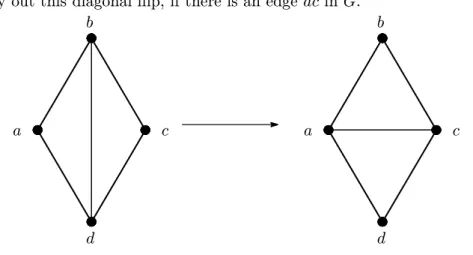
A diagonal °ip is an operation which replaces an edge e in the quadri- lateral D formed by two faces sharing e with another diagonal of D. A diagonal °ip can be applied only if the resulting graph is simple.

Wagner proved that any two spherical triangulations with the same num- ber of vertices can be transformed into each other by a sequence of diagonal

°ips, up to isomorphism [16]. For the torus, the projective plane and the

Klein bottle, Dewdney [4], Negami and Watanabe [10] proved the same

facts. Moreover, Negami [12] proved that for any surface F

, there exists

an integer N (F

) such that any two triangulations G and G

on F

can be

transformed into each other if j V (G) j = j V (G

) j ¸ N (F

). This result is

the origin of a big stream of the researches concerning with diagonal °ips in triangulations [13]. But there are only a few results on the number of diagonal °ips. Let us consider the minimum number of diagonal °ips needed to transformed one triangulation into the other.

From Wagner's proof, we can obtain the fact any two spherical triangu- lations with n vertices can be transformed into each other by at most O(n

) diagonal °ips. However, Komuro [7] proved that 8n ¡ 48 diagonal °ips are su±cient. We shall improve this result, focusing on a Hamilton cycle. Sup- pose that a spherical triangulation G has a Hamilton cycle C. Observe that G can decomposed into two spanning maximal outerplane graphs sharing C, and that each of the two maximal outerplane graphs can be transformed

into our standard form by at most max f n ¡ 5; 0 g diagonal °ips. Since we can prove that these procedures in the two graphs can be done in G inde- pendently, we can prove the following theorem, preserving C.

THEOREM1

Any two Hamiltonian triangulations on the sphere with n ver- tices can be transformed into each other by at most max f 4n ¡ 20; 0 g diagonal

°ips, preserving the existence of Hamilton cycles.

How can we transform a given triangulation on the sphere into one with

a Hamilton cycle? Tutte [15] has given a nice su±cient condition for plane

graphs to have Hamilton cycles as in the following theorem.

THEOREM 2

Every 4-connected plane graph has a Hamilton cycle.

In view of Theorem 2, let us estimate the number of diagonal °ips needed to transform a given triangulation G into a 4-connected one. Since every 3-cut in G lies on a separating 3-cycle in G, we want to break all 3-cycles by applying diagonal °ips. Since we can prove that every triangulation G on the sphere has at most n ¡ 4 separating 3-cycles and that each separating 3-cycle can be broken by a single diagonal °ip without creating a new 3-cut, we need at most n ¡ 4 diagonal °ips to transform G into a 4-connected one, and hence we have the following theorem by combining this and Theorem 1.

THEOREM 4

Any two triangulations on the sphere with n vertices can be transformed into each other by at most max f 6n ¡ 30; 0 g diagonal °ips, up to isomorphism.

We would like to extend this result to the projective plane. Similarly

to the spherical case, we observe that a contractible Hamilton cycle C in a

triangulation G on the projective plane decomposes G into a maximal outer

plane triangulation, and a triangulation on the MÄ obius band all of whose

vertices lie on the boundary, which is called a Catalan triangulation. Edel-

band with n vertices, and it was proved that any two of them can be trans- formed into each other by diagonal °ips, but the number of diagonal °ips had never been estimated in their paper. In Chapter 3, we estimated how many diagonal °ips su±ce to transform any two Catalan triangulations on the MÄobius band. Our theorem is the following.

THEOREM 13

Let G and G

be two triangulations on the projective plane with n vertices, each of which has a contractible Hamilton cycle. Then G and G

can be transformed into each other by at most 6n ¡ 12 diagonal °ips, preserving their Hamilton cycles.

Since Thomas and Yu [14] have proved that every 4-connected graph on the projective plane has a contractible Hamilton cycle and we can prove that a projective planar triangulation with n vertices has at most n ¡ 6 separating 3-cycles, we can prove the following theorem, which is the ¯rst result to give a linear bound for the minimum number of diagonal °ips to transform given two triangulations on a non-spherical surface with respect to n.

THEOREM 12

Any two triangulations on the projective plane with n ver- tices can be transformed into each other by at most 8n ¡ 26 diagonal °ips, up to isotopy.

In the second part, we would like to consider a linkage in triangulations

on surfaces. That is, we want to measure how rich linkage can be taken in a given triangulation. In order to do, we de¯ne an (m; n)-linkage of a graph, as follows. This notion is ¯rst de¯ned in [3].

We say that a graph G is (m; n)-linked if for any two disjoint subsets R and B of V (G) with j R j · m and j B j · n, there are two disjoint subgraphs G

and G

in G containing R and B, respectively. Note that when m = n = 2, the (2; 2)-linkage is equivalent to the 2-linkage, where a graph G is said to be k-linked if for any 2k distinct vertices s

; : : : ; s

, t

; : : : ; t

of G, there are k disjoint paths connecting s

and t

, for i = 1; : : : ; k. In Chapter 4, we prove the following theorem.

THEOREM 23

Let G be a planar graph with at least six vertices. Then G is (3; 3)-linked if and only if G is maximal and 4-connected.

In the above theorem, we can easily see that the maximality is necessary, since a graph with a non-triangular face is not 2-linked (hence it is not (2,2)- linked neither). So an essential argument to prove Theorem 23 is whether any spherical triangulation is (3; 3)-linked.

In Chapter 5, we shall generalize this result to triangulations on other

surfaces in terms of the connectivity of the graph and the representativity

of the embedding, where the representativity of an embedding G is the min-

imum number of intersecting points of G and any non-contractible simple closed curve on the surface. An essential argument in this generalization is that in a triangulation G, a minimal vertex cut lies on several cycles whose removal disconnects the surface. So, analyzing a relation between a mini- mal tree containing a speci¯ed vertex set S in G and a minimal cut set of G separating the tree, we obtain the following theorem, which also implies the su±ciency of Theorem 23 but whose proof is much shorter.

THEOREM 28

Let k be a positive integer. Every (k + 1)-connected b

c -

representative triangulation on any surface is (k; k)-linked.

Chapter 1

Foundation

In this chapter, we shall give the foundations of the thesis. That is, we shall present basic terminology and notation of graph theory and topology which will be needed in the following chapters.

1.1 Graphs

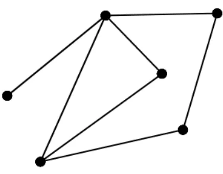
A graph G consists of a set V (G) of vertices, a set of E(G) of edges, and

a mapping associating to each edge e 2 E(G) an unordered pair x and y

of vertices called endpoints (or simply ends) of e. We say that an edge is

incident with its ends, and that it joins its ends. In this case, x and y are

called adjacent vertices of G. We allow x = y, in which the edge is called

Figure 1.1: Graphs

edges. The degree of a vertex x is the number of edges incident with x and is denoted by deg

(x). The set of vertices of G adjacent to a vertex x 2 V (G) is called the neighborhood of x in G and is denoted by N

(x).

A graph G is said to be simple if G has neither loops nor multiple edges, that is, there is no edge joining a vertex with itself and there is at most one edge between each pair of vertices of G. It is clear that for each x 2 V (G), deg

(x) = j N

(x) j if G is simple.

Two simple graphs G and G

are said to be isomorphic if there is a

bijection ½ : V (G) ! V (G

) such that for any x; y 2 V (G), xy 2 E(G)

if and only if ½(x)½(y) 2 E(G

). The bijection ½ is called an isomorphism

between G and G

.

1.2 Subgraphs and operations on graphs

We say that a graph K is a subgraph of G if V (K) ½ V (G) and E(K) ½ E(G). In particular, if V (G) = V (K), then K is a spanning subgraph of G.

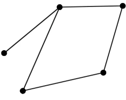
Let G be a graph, let K be a subgraph of G and let S be a nonempty subset of V (G). If V (K) = S and E(K) consists of the edges of G whose ends are both in S, then the subgraph K of G is said to be induced by S and is denoted h S i .

Figure 1.2: A induced subgraph of the graph in Fig: 5.1

We often construct new graphs from old ones by deleting or adding some vertices and edges. For a subset W of V (G), we de¯ne G ¡ W = h V (G) ¡ V (W ) i . Similarly, for a subgraph H of G, we de¯ne G ¡ H = h V (G) ¡ V (H) i .

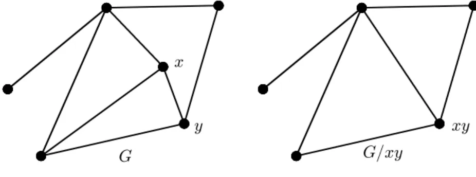
Given an edge xy of a graph G, the graph G=xy is obtained from G

by contracting the edge xy. To get G=xy, we identify the vertices x and y

and remove all resulting loops and multiple edges. A graph obtained by a

sequence of edge-contractions is called a contraction of G.

x

y xy

G G=xy

Figure 1.3: A graph G and its contraction G=xy

1.3 Paths and cycles

Let G be a graph and let

W := x

e

x

e

: : : e

x

where for x

2 V (G) and e

2 E(G), each e

joins x

and x

for i = 1; 2; : : : ; k. Then the sequence W is called a walk in G, and x

and x

are called the ends of W . The number k is called the length of W and denoted by j W j . If x

; : : : ; x

are all distinct, then W is called a path in G.

In a walk W = x

e

x

e

: : : e

x

, if x

= x

, then the walk W is

called closed. A closed walk W is called a cycle if x

; : : : ; x

are all distinct

and e

: : : ; e

are all distinct. We call a cycle of length k an k-cycle. A edge

x

x

is called a chord of C if x

x

2 = E(C) and x

; x

2 V (C). In particular, if C has no chord then we call it a chordless cycle.

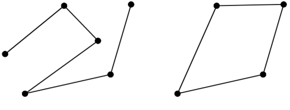
Figure 1.4: A path, A cycle

A cycle containing all vertices of a graph is called a Hamilton cycle. A graph G said to be a Hamiltonian if it has a Hamilton cycle.

1.4 Connectivity

A graph is connected if any two of its vertices can be joined by a path, and otherwise it is disconnected. A maximal connected subgraph of G is called a component of G. Let G be a connected graph and let S be a subset of V (G). If G ¡ S is disconnected, then S is called separating. In particular, if S ¡ f x g is not separating for any x 2 S, then S is called minimal.

Let G be a connected graph and let C be a subgraph of G. Let A be a

one of the components of G ¡ C and let x

; : : : ; x

2 V (C) be the vertices

adjacent to vertices of A. Then the connected subgraph consisting of A together with the edges joining A and f x

; : : : ; x

g is called a C-bridge with attachments x

; : : : ; x

. An edge xy 2 E(G) ¡ E(C) with x and y on C is also called a C-bridge with attachments x and y.

w

x

y

z

Figure 1.5: S

-bridge

Let G be a graph shown in Fig 1.5. Let S

= f x; y; z g ; S

= f x g and S

= f y; z g be subsets of V (G). Then

S

; S

; S

are separating

In particular, S

; S

are minimal.

Moreover

G ¡ f w g is one of S

-bridges with attachment x. Similarly, hf w; x gi is one of S

-bridges with attachment x.

1.5 Embedding of graphs into surfaces

Through this thesis, we shall call a connected compact 2-dimensional man-

ifold without boundaries a surface.

A closed curve on a closed surface F

is a continuous function ` : S

! F

or its image, where S

is the 1-dimensional sphere, that is, f (x; y) 2

j x

+ y

= 1 g . A closed curve ` is called simple if the function ` is an injection.

When we discuss embeddings of graphs into surfaces, we regard graphs as

1-dimensional topological spaces, not only as combinatorial objects. Roughly

speaking, to embed a graph into a surface F

is to draw the graph on F

without crossing edges. Sometimes, it is e®ective to regard an embedding as

an injective continuous map f : G ! F

. We deal with G and f(G) as the

same object intuitively. However, to distinguish G from the embedded one

f (G), we often call G an abstract graph while we call f (G) an embedding. In

this thesis, we often denote an embedded graph by G. When G is embedded

in a closed surface F

, then G can be regarded as a subset of F

. Each

component of F

¡ G is called a face of G embedded in F

. A closed walk

W of G which bounds a face F of G is called the boundary walk of F . An

embedded graph G is said to be a 2-cell embedding, or G is said to be 2-cell

embedded in F

if each face of G is homeomorphic to an open 2-cell, that is,

f (x; y) 2 R

j x

+ y

< 1 g . For a graph G embedded on a closed surface F

,

we denote the face set of G by F (G), and denote the vertex set and edge

sets of G by V (G) and E(G) respectively, as for abstract graphs. A graph

G is said to be planar if G is embeddable into the plane. If a graph G is a connected plane graph with all vertices lying on the boundary of its outer face, then we called an outerplane graph. Especially

if we cannot adding the edge preserving the condition of outerplane, then we called a maximal outerplane.

Let G

and G

be two graphs embedded in closed surfaces F

andF

, respectively. Two graphs G

and G

are said to be homeomorphic to each other if there exists a homeomorphism h : F

! F

with h(G

) = G

which induce an isomorphism from G

to G

. In this case, we also say that G

½ F

and G

½ F

are the same ones up to homeomorphism.

We say that a simple closed curve J on F

is trivial if J bounds a 2- cell on F

, and essential otherwise. We apply these de¯nitions to cycles of G by regarding them as simple closed curves on F

. The representativity of a graph G on a surface is the minimum number of intersecting points of G and `, where ` runs over all essential closed curves on the surface.

(For convenience, we de¯ne the representativity of a plane graph to be the in¯nity.) A graph G is said to be k-representative if the representativity of G is at least k.

A triangulation G of a surface F

is a simple graph embedded in F

so that each face of G is triangular and so that any two faces of G share

at most one edge. So it is easy to see every triangulation on any surface

is 3-connected and 3-representative. It is to see that a triangulation G is

k-representative if and only if every essential cycle of G has length at least k.

Chapter 2

Diagonal Transformations in Triangulations

In this chapter, we shall study the estimation problem for triangulations.

It will be shown that any two Hamiltonian triangulations with n vertices

on the sphere with n ¸ 5 vertices can be transformed into each other by

at most 4n ¡ 20. Moreover, using this result, we shall prove that at most

6n ¡ 30 diagonal °ips are needed for any two triangulations on the sphere

with n vertices to transform into each other.

2.1 Classical results

A triangulation G on a closed surface F

is a simple graph embedded on F

so that each face is triangular and any two faces meet along at most one edge. Let abd and bcd be two triangular faces of G which have an edge bd in common. The diagonal °ip of bd is to replace the diagonal bd with ac in the quadrilateral abcd (See Fiure 2.1). To avoid multiple edges, we do not carry out this diagonal °ip, if there is an edge ac in G.

a

b

c

d

a

b

c

d

Figure 2.1: Diagonal °ip

Classically, Wagner proved in [16] that any two triangulation on the

sphere with the same number of vertices can be transformed into each

other by a ¯nite sequence of diagonal °ips. Also, Dewdney [4], Negami

and Watanabe [10] have shown the same result for the torus, the projective

plane and the Klein bottle. The same fact does not hold for other sur-

faces in general, but Negami [12] has shown that there is a positive integer N = N (F

) for each surface F

such that two triangulations G

and G

can be transformed into each other by a ¯nite sequence of diagonal °ips if j V (G

) j = j V (G

) j > N . Moreover, there are several papers, for example [11], [2] and [1], describe interesting theorems on diagonal °ips.

2.2 The minimum number of diagonal °ips and the main theorem

From Wagner's proof, we can obtain the fact that any two spherical triangu- lations with n vertices can be transformed into each other by at most O(n

) diagonal °ips. However, Komuro [7] proved that 8n ¡ 48 diagonal °ips are su±cient, and he has constructed two spherical triangulations with n ver- tices which need at least 2n ¡ 15 diagonal °ips to transform into each other.

In the arguments on diagonal °ips in triangulations, the standard spherical triangulation with n vertices, denoted by ¢

, plays an essential role. (See Figure 2.2.) It is isomorphic to P

+ K

as a graph.

In this chapter, we focus on Hamiltonian spherical triangulations and consider diagonal °ips in those preserving the existence of Hamilton cycles:

THEOREM 1

Any two Hamiltonian triangulations on the sphere with n

Figure 2.2: Standard spherical triangulation ¢

vertices can be transformed into each other by at most max f 4n ¡ 20; 0 g di- agonal °ips, preserving the existence of Hamilton cycles.

Tutte [15] has given a nice su±cient condition for plane graphs to have Hamilton cycles as in the following theorem.

THEOREM 2 (Tutte[15])

Every 4-connected plane graph has a Hamilton cycle.

Theorem 2 asserts that the number of diagonal °ips needed to transform given two 4-connected spherical triangulations with n vertices is less than or equal to the number given in Theorem 1. Hence the following is obvious.

THEOREM 3

Any two 4-connected triangulations on the sphere with n ver-

tices can be transformed into each other by at most max f 4n ¡ 20; 0 g diagonal

Note that Theorem 3 does not always guarantee the 4-connecedness of the triangulations appearing in the process of diagonal °ips.

Finally, we shall prove the following theorem, estimating the number of diagonal °ips to transform a given spherical triangulation into a 4-connected graph. In particular, the estimation in Theorem 4 is better than Komuro's result.

THEOREM 4

Any two triangulations on the sphere with n vertices can be transformed into each other by at most max f 6n ¡ 30; 0 g diagonal °ips, up to isomorphism.

2.3 Hamiltonian triangulations on the sphere

We begin with the following lemmas each of which obviously holds.

LEMMA 5

For n=4; 5, there exists only one spherical triangulation with n vertices which are ¢

and ¢

, respectively.

LEMMA 6

Every maximal outerplane graph has a vertex of degree 2.

LEMMA 7

Every maximal outerplane graph with at least 5 vertices has a

vertex of degree at least 4.

LEMMA 8

Let G be a maximal outerplane graph with outer cycle C, and let e be any edge not contained in C. Then, e can be switched by a diagonal

°ip without breaking the simpleness of the graph.

Proof. Suppose that e = ac is a diagonal of a quadrilateral abcd, and it cannot be switched. Then b and d are adjacent in G. In this case, G has a subgraph isomorphic to K

with four vertices a; b; c and d. It is well-known that every outerplanar graph cannot include a subdivision of K

. Therefore, we get a contradiction.

Consider the maximal outerplane graph with n vertices isomorphic to P

+ K

. We call this the standard maximal outerplane graph and denote it by ¡

. The unique vertex of degree n ¡ 1 of ¡

is called the apex. (See

Figure 2.3) apex

Figure 2.3: Standard maximal outerplane graph ¡

PROPOSITION9

Let G be a Hamiltonian triangulation on the sphere with n vertices. Then G can be transformed into the standard spherical trian- gulation ¢

by at most max f 2n ¡ 10; 0 g diagonal °ips, up to isomorphism.

Moreover, if G is 4-connected, then at most max f 2n ¡ 11; 0 g diagonal °ips are enough.

Proof. Let G be a Hamiltonian triangulation on the sphere with a Hamilton cycle C. Suppose that j V (G) j = n. By Lemma 5, Thus, we may assume that n ¸ 6.

Clearly, G can be decomposed into two maximal outerplane graphs G

and G

such that G

\ G

= C. By Lemma 6, G

has a vertex v of degree 2.

Let v

and v

be the two neighbors of v in G

.

Now we turn attention into the situation around v in G

. Since deg

(v) ¸

3 by the 3-connectedness of G, we also have deg

(v) ¸ 3. (Here, if G is

4-connected, then we have deg

(v) ¸ 4.) If there is a triangular face vxy

in G

with xy = 2 E(C), then xy can be switched into vz in the quadri-

lateral vxyz formed by Lemma 8. Moreover, we have vz = 2 E(G

) since

deg

(v) = 2. Thus, the diagonal °ip replacing xy with vz does not break

the simpleness of the whole graph, either. Therefore, G

can be transformed

into the standard maximal outerplane graph S

» = ¡

with apex v by at most

n ¡ 4 diagonal °ips. (If G is 4-connected, then at most n ¡ 5 diagonal °ips

are enough.) Let G

be the Hamiltonian plane triangulation obtained from G by the sequence of diagonal °ips transforming G

into S

.

Now we consider the subgraph G

of G obtained by removing v. Then G

is G

= G ¡ f v g . We denote the outer cycle G

by C

. Since no two vertices of G

not adjacent in C

are adjacent in G

. We can freely apply a diagonal °ip for any edge not on C

, by Lemma 8.

In particular, since G

has at least 5 vertices, G

has a vertex u of degree at least 4, by Lemma 7. We can transform G

into the standard maximal outerplane graph S

» = ¡

with apex u by at most n ¡ 6 diagonal °ips, since deg

(u) ¸ 4 and deg

(u) = n ¡ 2. The resulting whole graph is nothing but the standard spherical triangulation ¢

. The number of diagonal °ips needed is at most 2n ¡ 10. (If G is 4-connected, then at most 2n ¡ 11 diagonal

°ips are enough.)

Note that no diagonal °ips are applied to the edges on the ¯xed Hamilton cycle C. Hence the existence of Hamilton cycles is always preserved in the process of diagonal °ips. Therefore, the proposition follows.

Now we shall prove Theorems 1 and 3.

Proof of Theorems 1 and 3. By Proposition 9, any two Hamiltonian trian-

gulations on the sphere with n vertices can be transformed into each other

by at most max f 4n ¡ 20; 0 g diagonal °ips, up to isomorphism, by the stan- dard spherical triangulation ¢

, preserving the existence of Hamilton cycles.

Moreover, if they are 4-connected, then at most max f 4n ¡ 22; 0 g diagonal

°ips are su±cient.

2.4 General spherical triangulations

In this section, we shall prove Theorem 4.

LEMMA 10

A spherical triangulation with n vertices has at most n-4 sep- arating 3-cycles.

Proof. Let G be a spherical triangulation with n vertices. We proceed by induction on n. In the case when n = 4, we have G = ¢

, by Lemma 5.

Since ¢

has no separating 3-cycle, the lemma hold, and hence we suppose that n ¸ 5.

We may assume that G has a separating 3-cycle C = xyz. Cutting

along C, we can decompose G into two spherical triangulations G

and G

such that G

\ G

= C. Let n

= j V (G

) j and n

= j V (G

) j , and hence

n = n

+ n

¡ 3. By the induction hypothesis, G

has at most n

¡ 4

separating cycles, and G

has at most n

¡ 4 separating cycles. Therefore

the number of separating cycles in G is at most

n

¡ 4 + n

¡ 4 + 1 = (n

+ n

¡ 3) ¡ 4 = n ¡ 4:

Thus the lemma follows for any n ¸ 4. (The standard spherical triangulation

¢

attains the equality.)

LEMMA 11

Let G be a spherical triangulation with n ¸ 6 vertices. Then G can be transformed into a 4-connected one by at most n ¡ 4 diagonal °ips.

Proof. It is easy to see that every spherical triangulation is 3-connected, and if f x; y; z g is a set of vertices such that G ¡ f x; y; z g , is disconnected, then x; y and z are contained in the same 3-cycle. Since G has at most n ¡ 4 separating 3-cycles by Lemma 10, we shall show that G has an edge e such that the diagonal °ip of e decreases the number of separating 3-cycles by at least one.

Let C = xyz be a separating 3-cycle in G and e = xy. We may suppose that if G has an edge included in at least two separating 3-cycles, then we choose such an edge as e. Let xayb be the quadrilateral formed by two triangular faces sharing e, where a and b lie in the interior and the exterior of C, respectively. Consider the cycle C in G has disappeared.

Now we show that no new separating 3-cycle has arisen in G

. Suppose

since every three vertices separating the graph lies on a 3-cycle. Hence we can put C

= abc. Since a was contained in a component of G ¡ f x; y; z g , we must have z = c. Since j V (G) j ¸ 6, either xza; yza; xzb or yzb is separating.

In these cases, xz or zy are included in at least two separating 3-cycles, but xy is contained in only one separating 3-cycle, which is contrary to the choice of e. Thus, no new separating 3-cycle has arisen in G

.

Now we shall prove Theorem 4.

Proof of Theorem 4. Let G

and G

be any two spherical triangulations with

n vertices. By Lemma 5, we may assume n ¸ 6. By Lemmas 10 and 11, for

i = 1; 2, G

can be transformed into a 4-connectde triangulation T

by at

most n ¡ 4 diagonal °ips. By Theorem 3, T

and T

can be transformed into

each other by at most 4n ¡ 22 diagonal °ips. Therefore, at most 6n ¡ 30

diagonal °ips can transform G

and G

into each other.

Chapter 3

Extension to the Projective Plane

In this chapter, we enhanced to the result in Chapter 2 to the projective plane. That is, we shall prove that any two triangulation on projective plane with n vertices can be transformed by a linear number of diagonal °ips with respect to n. This is the ¯rst result on non-spherical surfaces giving a linear bound for the number of diagonal °ips.

3.1 Main theorem

In this chapter, we shall prove the following theorem:

THEOREM 12

Any two triangulations on the projective plane with n ver- tices can be transformed into each other by at most 8n ¡ 26 diagonal °ips, up to isotopy.

A cycle C of a graph G is embedded in a closed surface F

is said to be contractible if C bounds a 2-cell on F

. In order to prove Theorem 3.1, we show the following theorem for triangulations on the projective plane with a contractible Hamilton cycle, as in the spherical case in Chapter 2.

THEOREM 13

Let G and G

be two triangulations on the projective plane with n vertices each of which has a contractible Hamilton cycle. Then G and G

can be transformed into each other by at most 6n ¡ 12 diagonal °ips, preserving their Hamilton cycles.

3.2 Triangulations with contractible Hamilton cy- cles

In the section, we deal only with triangulations which have contractible

Hamilton cycles. Clearly, a contractible Hamilton cycle in a triangulation G

on the projective plane separates G into two spanning subgraphs of G. One is

a maximal outerplane graph, denoted by G

, and the other is a triangulation

of the MÄ obius band, denoted by G

, in which all vertices appear on the

boundary of the MÄ obius band. We call it a Catalan triangulation on the MÄ obius band.

LEMMA 14

Let P be a maximal outerplane graph with n ¸ 3 vertices and let v be a vertex of degree k ¸ 2 in P . Then P can be transformed into a maximal outerplane graph in which the degree of v is exactly n ¡ 1, by exactly n ¡ k ¡ 1 ( · n ¡ 3) diagonal °ips, through maximal outer-plane graphs.

Proof. Let xy be an edge of P not in its outer cycle and let vxy and uxy be two faces sharing xy. Since deg

(v) = k, the number of vertices not adjacent to v is n ¡ k ¡ 1. Since P has no subgraph isomorphic to K

, u and v are not adjacent in P . Therefore, we can °ip xy without making multiple edges. Hence we can increase the degree of v one by one, by diagonal °ips.

Therefore, the lemma follows.

In [5], the Catalan triangulations on the MÄ obius band with n vertices were enumerated and it was proved that any two of them can be transformed into each other by diagonal °ips, but the number of diagonal °ips had never been estimated yet.

Let M

denote the MÄ obius band and let @M

denote the boundary

of M

. Let K be a Catalan triangulation on M

with m vertices. Let

v ; v ; : : : ; v be the vertices of K lying on @M

in this cyclic order. An

edge v

v

is said to be trivial if cutting along v

v

separates a disk D from M

. Clearly, the subgraph of K induced by the vertices on D is a maximal outerplane graph, which is said to be bounded by v

v

. Edges of K which are not trivial are said to be essential.

Suppose that a Catalan triangulation K on the MÄ obius band M

has no trivial edge. An essential edge e of K incident to a vertex of degree 3 is called a spoke. The subgraph of K induced by the essential edges which are not spokes is said to be the zigzag frame of K, which is uniquely taken. It is easy to see that the zigzag frame of K is a cycle of an odd length homotopic to the center line of M

. Moreover, if K has no trivial edge and no spoke, then K is 4-regular.

LEMMA 15

Let G be a triangulation on the projective plane with n ¸ 7 ver- tices. If G has a contractible Hamilton cycle C, then G can be transformed into K + K

by at most n ¡ 1 diagonal °ips, where K is some Catalan triangulation on the MÄ obius band.

Proof. Let G

and G

be the maximal outerplane graph and the Catalan triangulation on the MÄ obius band, each of which is a spanning subgraph of G with boundary C.

We shall make a vertex of degree 2 in G

by at most three diagonal

°ips, without breaking the simpleness of G. If G

has a trivial edge xy,

then xy bounds an outerplane graph L. It is easy to see that L has a vertex of degree 2 other than x and y. Thus, we have nothing to do, and hence we may suppose that G

has no trivial edge.

First, if G

has no trivial edge and no spoke, then G

is 4-regular.

Since G

is outerplanar, G

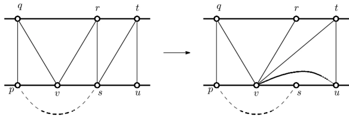
has a vertex of degree 2 in G

, say v with two neighbors p and s. Suppose that G

has faces pqv; qrv and rsv meeting at v, and faces vrs; rts and tus meeting at s in G

. (See the left-hand of Figure 3.1.) Observe that since deg

(v) = 2, any diagonal °ip in G

increasing the degree of v yields no edge forming multiple edges with an edge in G

. Moreover, since n ¸ 7, we have vt; vu = 2 E(G

); otherwise, we would have u = q and p = t. Therefore rs can be replaced with vt, and next st can be replaced with vu. Now s has degree 2 in the resulting graph on M

, which is obtained by two diagonal °ips. (See the right-hand of Figure 3.1.)

Finally suppose that G

has spokes but no trivial edges. We ¯rst sup-

pose that G

has two consecutive spokes pq and pr such that q and r are

adjacent on C and deg

(q) = deg

(r) = 3. Let pqs, pqr and prt be

three faces meeting at p. It is easy to see that a diagonal °ip can replace

an edge pq with sr without making multiple edges in G

, but G

might

already have an edge sr. In this case, by the planarity of G

, G does not

p

q r t

v s u p

q r t

v s u

Figure 3.1: Two diagonal °ips making a vertex of degree 2.

have an edge qt because of the obstruction of sr. Therefore, we can make r have degree 2 by one diagonal °ip.

Now consider the case when the vertices of degree 3 in G

are inde-

pendent. Since n ¸ 7, the zigzag frame of G

has length at least 5. (For

otherwise, i.e, if the zigzag frame has length 3 and all vertices of degree

3 are independent, then we have n · 6, a contradiction.) Let pq be a

spoke with deg

(q) = 3 and shared by two faces pqs and pqt. Note that

4 · deg

(s); deg

(t) · 5. Apply a diagonal °ip of pq to make a vertex

of degree 2 in G

. If impossible, G

already has an edge st. (Here, if G is

assumed to be 4-connected, then this does not happen, because G ¡ f p; s; t g

must be connected.) If G

has an edge st, then we can make q have degree

5 or 6 and s have degree 2 by at most three diagonal °ips, °ipping the edges

incident to s in G

, not on @M

, to make them be incident to q, similarly

to the case when G

is 4-regular. (Note that only the ¯nal case requires at most three diagonal °ips to make a vertex of degree 2 and it does not happen in the 4-connected case. Hence this proves the following remark.)

We turn our attention to G

. Let G

denote a Catalan triangulation with a vertex v of degree 2 obtained from G

by at most three diagonal

°ips. Then we can apply any diagonal °ip in G

increasing the degree of v, without making multiple edges with an edge of G

. Observe that deg

(v) ¸ 3, since every vertex of a triangulation on a closed surface has degree at least 3. Therefore, at most n ¡ 4 diagonal °ips can make v have degree n ¡ 1 in G

, by Lemma 14. In the resulting graph, v is adjacent to all other vertices, and the graph with v removed is obviously a Catalan triangulation with n ¡ 1 vertices.

As shown in the above proof, we have the following remark.

REMARK 16

In Lemma 15, if we assume the 4-connectedness of G, then the number of diagonal °ips can be improved to n ¡ 2.

3.3 General projective planar triangulations

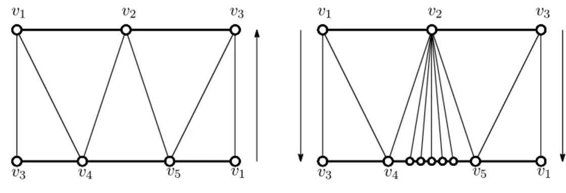
Consider a Catalan triangulation on the MÄ obius band shown in the left hand

of Figure 3.2, which is a unique Catalan triangulation with ¯ve vertices

isomorphic to K

. Let e = v

v

be an edge of the Catalan triangulation K

lying on the boundary of the MÄ obius band. Subdivide e by m vertices as shown in the right hand of Figure 3.2, where the MÄ obius band is obtained by identifying the arrows indicated in the left-hand and the right-hand sides of the rectangles. The resulting graph is called the standard form of the Catalan triangulations and denoted by ¡

.

v

v

v

v

v

v

v

v

v

v

v

v

v

v

Figure 3.2: K

and the standard form ¡

The following is the most essential argument in this chapter.

LEMMA 17

Every Catalan triangulation K on the MÄ obius band with n ver- tices can be transformed into the standard form ¡

by at most 2n ¡ 3 diagonal °ips.

Proof. Suppose that K has p trivial edges. Then it is easy to see that the

unique sub-Catalan triangulation, denoted by K

, of K with no trivial edges

is obtained from K by successively removing a vertex of degree 2. Clearly,

K

has exactly n ¡ p vertices.

Suppose that K

has q spokes and let r = n ¡ p ¡ q. Then the zigzag frame v

¢ ¢ ¢ v

, of K

has an odd length r ¸ 3. Let q

be the number of spokes of K

incident to v

, for i = 1; : : : ; r. We may suppose that q

+ q

+ ¢ ¢ ¢ + q

¸ q

+ q

+ ¢ ¢ ¢ + q

. (For otherwise, we can replace v

by v

for each i, because the subscripts are cyclic and taken modulo r). Let q

+ q

+ ¢ ¢ ¢ + q

= m and hence we have 2m · q. (See Figure 3.3.)

v

v

v

v

v

v

v

v

v

v

v

v

v

Figure 3.3: K

with zigzag frame v

v

: : : v

If r = 3, then by the simpleness of graphs, we have q

; q

¸ 1. Hence we can °ip an edge v

v

to make the zigzag frame have length 5. So, suppose that r ¸ 5. Apply diagonal °ips to all m spokes incident to v

; v

; : : : ; v

to make them trivial one by one. The number of diagonal °ips we did is exactly

q

+ q

+ ¢ ¢ ¢ + q

= m: (3.1)

Note that even if r = 3, the estimation (1) is true. Though we need one more diagonal °ip of v

v

to increase the length of the zigzag frame, this diagonal °ip decreases q

and q

by one, respectively.

Next reduce the length of the zigzag frame from r to 5. In particular, we ¯rst apply a diagonal °ip of v

v

, secondly °ip q

spokes incident to v

, and ¯nally °ip v

v

. (See Figure 3.4(1).) The number of diagonal °ips we did is q

+ 2. In the resulting graph, the zigzag frame has length r ¡ 2, and exactly one new trivial edge v

v

appears. As far as that the length of the zigzag frame is at least 7, we apply these operations. If its length is exactly 5, then we apply q

+ q

diagonal °ips, as shown in Figure 3.4(2). Then the total number of diagonal °ips we did is

(q

+ 2) + (q

+ 2) + ¢ ¢ ¢ + (q

+ 2) + q

+ q

· (q ¡ m) + 2

µ

r ¡ 5 2

¶

: (3.2)

Let H

be the current Catalan triangulation obtained from K

. The

zigzag frame of H

has length exactly 5, and all spokes of H

are incident

to v

. Moreover, H

has

(r ¡ 5) + m trivial edges, since all m spokes

incident to v

; v

; : : : ; v

in K

are replaced with trivial edges of H

, and

since decreasing the length of the zigzag frame of K

by two yields exactly

one new trivial edge. Let H be the Catalan triangulation consisting of H

and all trivial edges of K. Then H has exactly p +

(r ¡ 5) + m trivial edges.

v

v

v

v

v

(1)

v

v

v

v

v

(2)

v

v

v

v

v

v

v

v

v

v

v

v

v

v

v

v

v

v

v

v

Figure 3.4: Reducing the length of zigzag frame.

Now, renaming vertices, we put H with the zigzag frame u

u

u

u

u

as shown in Figure 3.5, where u

= v

; u

= v

and u

= v

. The four triangular faces u

u

u

; u

u

u

; u

u

u

and u

u

u

of H come from K

. Let R

denote the outer-plane graph bounded by an edge u

u

and containing the edge u

u

, for i 6 = 3. (Note that R

might be just an edge.)

The region F

of the zigzag frame of H is the union of the faces bounded

by the two edges u

u

; u

u

and the path on @M

connecting u

and

u

, for each i, where the subscripts are taken modulo 5. Now we shall

transform H into a Catalan triangulation in which all the regions of the

zigzag frame, except one corresponding to F

, consists of just one face.

u

u

u

u

u

u

u

R

R

R

R

Figure 3.5: The Catalan triangulation H.

Here we focus on the outer-plane graph R

and ¯rst suppose that j V (R

) j ¸ 3. By Lemma 14, we can make u

have degree j V (R

) j ¡ 1 by at most j V (R

) j ¡ 3 diagonal °ips. Let u

; x

; : : : ; x

; u

be the vertices of R

lying on @M

in this order. Apply ¯ve diagonal °ips of u

u

, u

u

, u

x

, u

u

and u

u

in this order, if l ¸ 2. (See Figure 3.6.) If l = 1, then apply three diagonal °ips of u

u

, u

u

, u

u

in this order. In the resulting graph, each of two regions of the zigzag frame corresponding to F

and F

is just a face.

The number of diagonal °ips we did is at most j V (R

) j ¡ 3 + 5.

Secondly we suppose that j V (R

) j = 2. If we also have j V (R

) j = 2, then we have nothing to do for F

and F

. So, suppose that j V (R

) j ¸ 3.

Similarly to the above case, at most j V (R

) j ¡ 3 diagonal °ips make u

have

degree j V (R

) j ¡ 1 in R

and we apply two diagonal °ips of u

u

and u

u

.

u

u

u

u

u

x

u

R

u

u

u

u

u

x

u

R

Figure 3.6: Moving vertices of R

and R

.

In the resulting graph, the two regions corresponding to F

and F

are just faces. Then the number of diagonal °ips we did is at most j V (R

) j ¡ 3 + 2.

Note that by the above operations, the number of trivial edges decreases by one, if j V (R

) j ¸ 3 or j V (R

) j ¸ 3.

We can do the same procedures for the regions R

and R

. Let L denote the resulting graph in which exactly four regions are just faces. Hence, the number of diagonal °ips transforming H into L is at most

max fj V (R

) j + 2; j V (R

) j ¡ 1 g + max fj V (R

) j + 2; j V (R

) j ¡ 1 g

· p + 1

2 (r ¡ 5) + m + 8; (3.3)

since

( j V (R

) j¡ 2)+( j V (R

) j¡ 2)+( j V (R

) j¡ 2)+( j V (R

) j¡ 2) · p+ 1

2 (r ¡ 5)+m:

Note that we can assume that the number of trivial edges of L is at most

R

and R

has at least three vertices. (For otherwise, we don't need to add (3.3) to the estimation of the maximum number of diagonal °ips, and this case requires a few number of diagonal °ips.)

Finally we °ip all trivial edges of L, all of which are incident to u

. Since the number of trivial edges of L is at most p +

(r ¡ 5) + m ¡ 1, the number of diagonal °ips transforming L into the standard form is at most

p + 1

2 (r ¡ 5) + m ¡ 1 = p + r

2 + m ¡ 7

2 : (3.4)

Therefore, by (3.1),(3.2),(3.3) and (3.4), the total number of diagonal

°ips is at most

m + (q ¡ m + r ¡ 5) +

p + r

2 + m + 11 2

¶

+

µ

p + r

2 + m ¡ 7 2

¶

= 2p + q + 2m + 2r ¡ 3 · 2(p + q + r) ¡ 3 = 2n ¡ 3;

since q ¸ 2m. Therefore, the lemma follows.

3.4 Triangulations on the projective plane with contractible Hamilton cycles

In the previous section, we described only the result on triangulations with

contractible Hamilton cycles. In this section, we shall mention how we can

obtain triangulations with contractible Hamilton cycles from any triangula- tions.

The following gives an important su±cient condition for a graph on the projective plane to have a contractible Hamilton cycle.

LEMMA 18 (Thomas and Yu [14])

Every 4-connected graph on the pro- jective plane has a contractible Hamilton cycle.

The following lemma is essential.

LEMMA 19

Let G be a triangulation on the projective plane with n vertices.

Then G can be transformed into a 4-connected triangulation by at most n ¡ 6 diagonal °ips.

Proof. Observe that a triangulation on the projective plane has no separating 3-cycle if and only if it is 4-connected. We ¯rst show that G has at most n ¡ 6 separating 3-cycles, by induction on n. It is well-known that the smallest triangulation on the projective plane is the unique triangular embedding of K

, which has no separating 3-cycle. Therefore, the lemma holds when n = 6.

When n ¸ 7, we may assume that G has a separating 3-cycle C =

xyz, and it is innermost, that is, there is no separating 3-cycle in the 2-

triangulation G

with no separating 3-cycle and a triangulation G

on the projective plane. By induction hypothesis, G

has at most j V (G

) j ¡ 6 separating 3-cycles. Let M denote the number of separating 3-cycles in G.

Then we have

M · j V (G

) j ¡ 6 + 1 = (n ¡ j V (G

) j + 3) ¡ 5 · n ¡ 6;

since j V (G

) j ¸ 4.

Now we shall show that there is a diagonal °ip decreasing the number of separating 3-cycles by at least one. Let C = xyz be a separating 3-cycle in G and e = xy. Let xayb be the quadrilateral formed by two triangular faces sharing e, where a lies in the 2-cell region bounded by C. Consider the diagonal °ip of e replacing xy with ab. In the resulting graph G

, the separating cycle C in G has disappeared.

We shall show that no new separating 3-cycle arises in G

, by possibly

re-choosing e. Suppose that G

has a new separating 3-cycle C

. Then C

contains both a and b; otherwise, C

would be contained in G. We must have

C

= abz, where we assume that x is contained in the 2-cell region bounded

by C

in G

. This means that V (G

) = f x; y; z; a g since C is innermost in

G. In this case, the edge yz can be °ipped to destroy a 3-cycle byz and

make no new separating 3-cycle, because byz separates a and other vertices

outside byz. Therefore, at most n ¡ 6 diagonal °ips can make the graph be

4-connected.

3.5 Proof of theorems

It is well-known that the smallest triangulation on the projective plane is the unique triangular embedding of K

. Let xy be one of its edges, and suppose that two faces xyz and xyw share xy. Subdivide xy by m vertices v

; : : : ; v

and add 2m edges v

z; v

w for i = 1; : : : ; m. The resulting graph with m + 6 vertices is called the standard form of triangulations on the projective plane and denoted by ª

. (See Figure 3.7.) Clearly, we obtain the standard form ª

from the standard form §

of Catalan triangulations of the MÄ obius band M

by pasting a disk along @M

, placing a vertex v at its center and joining v to all vertices of §

.

We ¯rst prove the following theorem.

THEOREM 20

Let G be a triangulation on the projective plane with n ver- tices which has a contractible Hamilton cycle. Then G can be transformed into ª

, preserving the Hamilton cycle, by at most 3n ¡ 6 diagonal °ips.

If G is 4-connected, then the number of diagonal °ips is improved to 3n ¡ 7.

Proof. We may suppose that n ¸ 7. By Lemma 15, G can be transformed

Figure 3.7: The standard form ª

of triangulations on the projective plane.

where K is some Catalan triangulation on the MÄ obius band with n ¡ 1 vertices. (By Remark 16, if G is 4-connected, the number \n ¡ 1" of diagonal

°ips can be replaced with \n ¡ 2".)

Note that no two vertices of K are joined by an edge outside K. There- fore, it su±ces to prove that K can be transformed into §

. By Lemma 17, it can be done by at most 2(n ¡ 1) ¡ 3 diagonal °ips. Therefore, G can be transformed into ª

by at most 3n ¡ 6 (3n ¡ 7 when G is 4-connected) diagonal °ips, preserving the Hamilton cycle.

THEOREM 21

Every triangulation on the projective plane with n vertices can be transformed into the standard form ª

by at most 4n ¡ 13 diagonal

°ips, up to isotopy.