H∞ control system design attenuating initial state uncertainties: Evaluation by a magnetic suspension system
著者 Namerikawa Toru, Fujita Masayuki, Smith Roy S.
journal or
publication title
Proceedings of the IEEE Conference on Decision and Control
volume 1
number 87
page range 92
year 2001‑01‑01
URL http://hdl.handle.net/2297/6743
1
Initial State Uncertainties :
Evaluation by a Magnetic Suspension System
Toru Namerikawayz, Masayuki Fujitay and Roy S. Smithz
y Departmentof Electrical and Electronic Engineering
KanazawaUniversity
E-mail: ftoru, [email protected]
z Departmentof Electrical and Computer Engineering
University of California,Santa Barbara
E-mail: [email protected]
Abstract
ThispaperdealswithanH
1
controlattenuatinginitial-
state uncertainties, and its application to a magnetic
suspension system. An H
1
control problem, which
treats a mixed attenuation of disturbance and initial-
state uncertainty for linear time-invariant systems in
the innite-horizon case, is examined. The mixed at-
tenuationsuppliesH
1
controlswithgoodtransientsor
assures H
1
controls of robustnessagainst initial-state
uncertainty. Weapply this methodto amagnetic sus-
pension system, and evaluate attenuation property of
the proposed disturbance and initial-state uncertainty
viasimulationsandexperiments.
keywords: H
1
Control, DIA Control, Initial-State
Uncertainties,MagneticSuspensionSystems
1 Introduction
Mixedattenuationsofdisturbancesandinitialstateun-
certainties are expected to supply H
1
control prob-
lem withsomegoodtransientproperties. Inthenite-
horizoncase,ageneralizedtypeofH
1
controlproblem
which formulated and solved by Uchida and Fujita[1]
and Khargonekaretal.[2]. This problemwasextended
to the innite-horizon case, and a generalized type of
H
1
control problem which considers a mixed atten-
uation of disturbance and initial-state uncertainty in
the innite-horizon case was derived by Uchida and
authors[3]. In thispaper,weevaluatetheeectiveness
of the proposed approach[3] with a magnetic suspen-
sion system viasimulations and experiments. A mag-
netic suspension systemcansuspend amagnetic body
by magnetic forces without any contact[4]. Feedback
control,especiallyrobustfeedbackcontrolisindispens-
ablefor amagneticsuspensionsystem, which isessen-
tially an unstable system. Recently, this seems to be
showthat theproposed controllerhasarelativelybet-
ter transientproperty than the conventional standard
H
1
controller. Next, a role of the weighting matrix
N forthe initial statex
0
is shown via numerical sim-
ulation. N is a measure of relative importance of the
initial-stateuncertaintyattenuationto thedisturbance
attenuation. Finally,usefulnessandeectiveness ofthe
free parameter of the mixed attenuation of distur-
bance andinitial-stateuncertaintyisexamined viaex-
periments.
2 Mixed attenuation ofdisturbance and
initial-state uncertainties
Considerthe lineartime-invariantsystem which is de-
nedonthetimeinterval[0;1)anddescribedby
_
x = Ax+Bu+Dv; x( 0)=x
0
y = Cx+w
z = Fx
(1)
where x 2 R n
is the state and x
0
is the initial state;
u 2 R r
is the control input; y 2 R m
is the observed
output; g :=(z 0
u 0
) 0
2R q+r
isthe controlled output;
h := (v 0
w 0
) 0
2 R p+m
is the disturbance. Without
lossof generality, we regardx
0
as the initial-stateun-
certainty, andx
0
=0asknowninitial-statecase. Each
element of the disturbance h(t) is a square integrable
functiondened on[0;1); A,B,C, D andF arecon-
stant matrices of appropriate dimensions and satises
that ( C ;A;B) and ( F;A;D) are controllable and ob-
servable. Forsystem (1),everyadmissiblecontrolu(t)
isgivenbyalineartime-invariantsystemoftheform
u=Js+Ky; s_=Gs+Hy; s(0)=0 (2)
which makestheclosed-loopsystemgivenby (1) and
(2)internallystable, wheres(t)isthestateofthecon-
trollerofanitedimension;J,K,GandHareconstant
attenuatingdisturbancesandinitialstateuncertainties
in thewaythat,forgivenN >0,g=( z 0
;u 0
) 0
satises
kgk 2
2
<khk 2
2 +x
0
0 N
1
x
0
(3)
for all h = ( v 0
;w 0
) 0
2 L 2
[0;1) and all x
0 2 R
n
, s.t.,
( v;w;x
0
)6= 0. We call such an admissiblecontrol the
disturbance and initial state uncertainty attenuation
(DIA) control.
2.1 DIAControl
In order to solve theDIA control problem, werequire
theso-calledRiccatiequationconditions:
A1 : There exists a solution M > 0 to the Riccati
equation
MA+A 0
M+F 0
F M(MM 0
DD 0
)M=0 (4)
suchthatA BB 0
M+DD 0
M isstable.
A2 : There exists a solution P > 0 to the Riccati
equation
PA 0
+AP+DD 0
P( C 0
C F
0
F)P =0 (5)
suchthatA PC 0
C+PF 0
F isstable.
A3 : (PM)<1,
where (X) denotes the spectral radius of matrix X,
and (X)=maxj
i ( X)j.
Inadditiontotheseconditions,letusintroducethefol-
lowingcondition:
A4 : Q+N 1
P 1
> 0 where Q is the maximal
solutionoftheRiccatiequation
Q A+DD 0
P 1
+ A+DD 0
P 1
0
Q
Q(DD 0
+LPC 0
CPL 0
)Q=0
(6)
withL:=(I PM) 1
.
Theorem 1 [3 ] Suppose that the conditions (A1),
(A2), and (A3) are satised. The central control (7)
is a DIA control if and only if the condition (A4) is
satised, wherethe central control isgiven by
u = B
0
Sx (7)
_
x = Ax+Bu+PC 0
( y Cx )+PF 0
Fx ;
x(0)=0; S :=M(I PM) 1
:
2.2 Parameterization of allDIA Controllers
Under theassumptionthat(A1)-(A3)aresatised,the
class of all H
1
controls u(t)are parametrized with a
parameter as
u(t) = u(t)+
y y
(t) (8)
u(t) = B 0
Sx; y(t)=C(I+PS)x
_
x(t) = (A BB 0
S PC 0
C+PF 0
F)x
0
fer function representation (s), s.t. jj wjj 2
2
<
jjwjj 2
2
; 8w6=02L 2
[0;1).
Theorem2 [3 ]Supposethattheconditions(A1)-(A3)
aresatised. AnH
1
control (8)withaparameter (s)
isaDIAcontrol ifandonly if
Q
22 +N
1
P 1
>0 (10)
where Q
22
is the (2;2) block of the maximal solution
Q=
Q
11 Q
12
Q 0
12 Q
22
, whose existence is assured, of the
Riccati equation
Q
A
m
0
PSBKm A+DD 0
P 1
+
Am 0
PSBK
m
A+DD 0
P 1
0
Q
Q
BmB 0
m
BmCPL 0
LPC 0
B 0
m DD
0
+LPC 0
CPL 0
Q
K 0
m K
m 0
0 0
=0 (11)
foraminimalrealization( A
m
;B
m
;K
m
)of (s) ,where
A
m
is stable, and L =(I PM) 1
. Q
22
is given in-
dependent ofa particular choiceof realization of (s),
andQ
22 0.
3 SystemDescriptionand Modeling
Magneticsuspensionsystemscansuspendobjectswith-
out any contact. Increasing use of this technology is
nowutilizedforvariousindustrialpurposes,andhasal-
ready applied to magneticallylevitated vehicles, mag-
neticbearings,etc.
3.1 Construction
TheexperimentalsetupisshowninFig.1[4]. Anelectro-
magnetislocatedatthetopoftheexperimentalsystem.
Thecontrol problem is to levitatethe iron ball stably
utilizingtheelectromagnetic force,where amassM of
the iron ball is 1:75 kg, and steady state gap X is 5
mm. Note that thissimpleelectromagnetic suspension
system requires feedback control in order to bework-
able. As agap sensor, a standard induction probe of
eddycurrenttypeis placedbelowtheball.
3.2 Mathematical Model
In order to derive a model of the system by physical
laws,weintroducefollowingassumptions[4].
[a1] Magnetic ux density and magnetic eld donot
haveanyhysteresis,and theyarenotsaturated.
X+x
f
Mg
Iron ball L R
Electromagnet I+i
E+e
Gap sensor
Figure1: MagneticSuspensionSystem(M.S.S.)
[a3] Magneticpermeabilityoftheelectromagnetisin-
nity.
[a4] Eddy current in the magnetic pole can be ne-
glected.
[a5] Coilinductanceis constantaroundtheoperating
point,andanelectromotiveforceduetoamotion
oftheironballcanbeneglected.
These assumptions are almost essential to model this
system. Undertheseassumptions,wederivedequations
of themotion, theelectromagnetic force, andthe elec-
triccircuitas
M d
2
x
dt 2
= Mg f+v
m
; (12)
f = k
I +i
X+x+x
0
2
; (13)
L di
dt
+R (I+i) = E+e+v
L
; (14)
where M is amassofthe ironball, X is asteadygap
betweentheelectromagnet(EM)andtheironball,xisa
deviationfromX,I isasteadycurrent,iisadeviation
from I, E is a steady voltage, e is a deviation from
E, f is EM force, k, x
0
are coeÆcients of f, L is an
inductanceofEM,andRisaresistanceofEM,v
m and
v
L
areexogenousdisturbanceinputs.
Nextwelinearizetheelectromagneticforce(13)around
theoperatingpointbytheTaylorseriesexpansionas
f =k
I
X+x
0
2
K
x x+K
i
i; (15)
where K
x
=2kI 2
=(X+x
0 )
3
andK
i
=2kI=(X+x
0 )
2
.
The sensor provides the information for the gap x(t).
Hence themeasurementequationcanbewritten as
y=x+w (16)
wherewrepresentsthesensornoiseaswellasthemodel
uncertainties. Thus,summinguptheaboveresults,the
stateequationsforthesystemare
_ x
g
= A
g x
g +B
g u
g +D
g v
0
y
g
= C
g x
g +w
(17)
wherex
g
:=[x x_ i]
0
,u
g :=e,v
0 :=[v
m v
L ]
0
,
A
g
= 2
4
0 1 0
4481 0 18:4
0 0 45:7
3
5
; B
g
=
0 0 1:97
0
C
g
=
1 0 0
; D
g
= 2
4
0 0
0:57 0
0 1:97 3
5
Here (A
g
; B
g
) and (A
g
; D
g
) are controllable, and
(A
g
; C
g
)isobservable.
4 Control SystemDesign
4.1 Problem Setup
Forthemagneticsuspensionsystemdescribedandmod-
eledintheprevioussection,ourprincipalcontrolobjec-
tiveisitsstabilization. Further,aswehaveclariedin
the modeling of the disturbances, it should be stabi-
lized robustly against 1) unmodeled dynamics, 2) the
neglected nonlinearities, 3) the parametric uncertain-
ties. To this end, we will setup the control problem
withintheframeworkoftheH
1
DIAcontrol.
First let us consider the systemdisturbance v
0 . Since
v
0
mainly actsontheplantinalowfrequencyrangein
practice,itishelpfultointroduceafrequencyweighting
factor. Hence letv
0
beoftheform
v
0
= W
1
(s)v(s) (18)
W
1
(s) = W(s)=C
w1
(sI A
w1 )
1
B
w1
= [1 1] 0
whereW
1
(s)isafrequencyweightingwhosegainisrel-
ativelylargein alowfrequencyrange. Thesevalues,as
yet unspecied, canberegardedasfreedesign param-
eters. Next we consider the variables which we want
to regulate. In this study, since our main concern is
in the stabilization of the iron ball, the gap and the
correspondingvelocityarechosen;i.e.,
z
g
=F
g x
g
; F
g
=
1 0 0
0 1 0
(19)
Then,astheerrorvector,letus deneasfollows
z=z
g
; =diag
1
2
(20)
where is a weighting matrix on the regulated vari-
ables z
g
. This value, as yet unspecied, are also free
designparameters. Finally,letx:=[x x ] 0
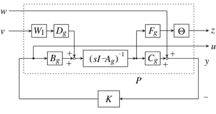
, where
Fg
W1 Dg
sI Ag
( )1 Cg
Θ Bg
K P w
v z
u + y
+
+ +
Figure2: GeneralizedPlant
x
w1
denotesthestateofthefrequencyweightingW
1 (s),
then we can construct the generalized plantas in the
following;
_
x = Ax+Bu+Dv
y = Cx+w
z = Fx (21)
where
A =
A
g D
g C
w1
0 A
w1
; B=
B
g
0
C =
C
g 0
; D=
D
g D
w1
B
w1
; F =
F
g 0
Theblockdiagramofthegeneralizedplantwithanun-
speciedcontrollerK is shown inFig.2. Sincethedis-
turbances v and w representthe various model uncer-
tainties, the eects of these disturbances on the error
vectorz shouldbereduced.
Now our control problem setup is: nd an admissible
controllerK(s)thatattenuatesdisturbancesandinitial
stateuncertaintiestoachieveDIAconditionin (3).
4.2 Design I:Central Controller
We design controllers for the generalized plant in the
previoussubsection basedonthe following4-Steppro-
cedure.
[Step 1] Selection of the frequency weighting
functionW(s) : W
1
(s)isafrequencyweightingwhose
gainisrelativelylargeinalowfrequencyrange.
[Step 2]Selectionof the weightingMatrix :
is aweightingmatrixontheregulatedvariablesz
g .
[Step3]Constructionofgeneralizedplant: With
the specied design parameters in Steps 1 and 2, the
generalizedplantisconstructed. TheDIAcontrolleris
designedforthisplant.
[Step 4] Calculation of the maximum matrix
N: Calculate themaximumN satises thecondition
(A4). For the sake of simplicity, the structure of the
matrix N is limited in N =nI, where n is apositive
scalarnumber.
4.2.1 DIAController 1: Aftersomeiteration
inMATLABenvironment,theseparametersarechosen
asfollows;
W
1 (s)=
7:5
s+1:0e 4
; =diag
1:01 1:0e 5
(22)
Directcalculationsyieldthecentralcontroller;
K
DIA
1
=C
f1 (sI A
f1 )
1
B
f1
(23)
where
A
f1
= A BB
0
S PC
0
C+PF 0
F
= 2
6
6
4
1:38e 2
1:00 0 0
4:48e 3
2:98e 3
1:84e 1
4:28
1:05e 11
1:98e 7
2:72e 4
6:33e 3
4:06e 2
2:71e 8
0 1e
4 3
7
7
5
B
f1
= PC 0
=
2:11e 9
1:41e 11
2:07e 5
6:39e 5
T
C
f1
= B
0
S
=
1:68e 5
3:18e 1
4:36e 2
1:01e 2
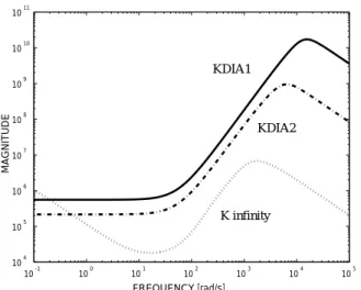
The frequency response of the controller K
DIA1 is
showninFig. 3byasolidline. Andthemaximumvalue
oftheweightingmatrixN isN =3:85510 9
I. We
designedthe standard H
1
controller for the compari-
son, where the H
1
controller[4] wasdesigned via the
MATLAB commandhinfsyn.m. Wedenotethestate-
spacerealizationoftheobtainedH
1
controlleras K
1 .
Thefrequencyresponseof the controllerK
1
is shown
inFig. 3byadottedline.
Comparingthe controllers K
1 and K
DIA1
, simulated
stepresponses of these twocontrollersfrom the initial
state x
02
= [x;x ;_ i]
0
= [0; 0; 0:1]
0
are shown in Fig.4,
wherethe solidline showsaresponse withK
DIA
1 and
the dashed line shows one with K
1
. From this re-
sult,wecanseethatK
DIA
1
achievesbetterperformance
againstinitial stateuncertaintythanK
1 does.
4.2.2 Investigation of Weight N: The
weighting matrix N on x
0
is a measure of relative
importance of theinitial-state uncertainty attenuation
to the disturbance attenuation. A larger choice of N
in the sense of matrix inequality order means nding
anadmissible controlwhichattenuatestheinitial-state
uncertainty more. For the evaluation of feedback
performance against theweightingmatrix N, we have
designed another DIA controller K
DIA
2
. After some
iterationin MATLAB environment, designparameters
arechosenasfollowstoobtainanotherDIAcontroller;
W
1 (s)=
6:75
s+1:0e 4
; =diag
1:025 1:0e 4
(24)
Direct calculations yield thecentral controllerK
DIA
2 ,
anditsfrequencyresponseisshowninFig. 3byadash-
dotline.
ThemaximumvalueofNsofthecontrollersK
DIA1 and
K
DIA2
aregivenin Table1.