EnhancingthePerformanceofCuckooSearchAlgorithmwithMulti-LearningStrategies PAPER

(1)

PAPER

Enhancing the Performance of Cuckoo Search Algorithm with Multi-Learning Strategies

Li HUANG^†,††^a), Xiao ZHENG^†††^b), Shuai DING^†^c),Nonmembers, Zhi LIU^††††^d),Member, andJun HUANG^†††^e),Nonmember

SUMMARY The Cuckoo Search (CS) is apt to be trapped in local optimum relating to complex target functions. This drawback has been rec- ognized as the bottleneck of its widespread use. This paper, with the pur- pose of improving CS, puts forward a Cuckoo Search algorithm featur- ing Multi-Learning Strategies (LSCS). In LSCS, the Converted Learning Module, which features the Comprehensive Learning Strategy and Opti- mal Learning Strategy, tries to make a coordinated cooperation between exploration and exploitation, and the switching in this part is decided by the transition probabilityPc. When the nest fails to be renewed afterm iterations, the Elite Learning Perturbation Module provides extra diversity for the current nest, and it can avoid stagnation. The Boundary Handling Approach adjusted by Gauss map is utilized to reset the location of nest beyond the boundary. The proposed algorithm is evaluated by two diﬀer- ent tests: Test Group A(ten simple unimodal and multimodal functions) and Test Group B(the CEC2013 test suite). Experiments results show that LSCS demonstrates significant advantages in terms of convergence speed and optimization capability in solving complex problems.

key words: multi-learning strategy, cuckoo search, bound handling mech- anism, elite learning

1. Introduction

In tackling objective functions which are distinguishable and continuous, especially those with large size characteristics, metaheuristics-based algorithms are usually justified as a robust and powerful solution, and this kind of algorithm is generally believed to be superior to the traditional optimization. Inspired by the unique characteristics of the cuckoos, the standard Cuckoo Search (CS) algorithm[1] is catego- rized as metaheuristics. Its rules state that each host has a probability of discovering an alien egg, and if the probability is greater than a switching parameterPa, the host will find the alien egg and will build a new nest in a new location.

Manuscript received January 15, 2019.

Manuscript revised May 31, 2019.

Manuscript publicized July 9, 2019.

†The authors are with School of Management, Hefei Univer- sity of Technology, Hefei 230009, Anhui, P.R. China.

††The author is with School of Management Science and Engi- neering, Anhui University of Technology, Maanshan, P.R. China.

†††The authors are with the School of Computer Science and Technology, Anhui University of Technology, China.

††††The author is with the Department of Mathematical and Systems Engineering, Shizuoka University, Hamamatsu-shi, 432–

8561 Japan.

a) E-mail: [email protected] (Corresponding author) b) E-mail: [email protected] (Corresponding author) c) E-mail: [email protected]

d) E-mail: [email protected] e) E-mail: huangjun [email protected]

DOI: 10.1587/transinf.2019EDP7013

Different from such metaheuristic algorithms as the genetic algorithm (GA)[2],[3]and the particle swarm optimization (PSO)[4]–[6], the standard Cuckoo Search (CS) algorithm has distinguished itself with its reference to the L´evy Flight which features a heavy-tailed probability distribution, and which application in the global random walk makes the algorithm more effective. In solving a unimodal function, the global random walk of the CS algorithm will quicken speed at which each nest moving to the global optimal nest. How- ever, in solving more complex functions, the global random walk is at the risk of excessive exploitation[7], which occurs when a nest loses its global exploration capacity within a few iterations, and thus makes the standard CS algorithm be prone to premature convergence, and makes nest baffled in pursuing local optimal[8].Thus, the standard CS algorithm is prone to premature convergence, and makes nest baffled in pursuing local optima.

To improve the performance of the standard CS algorithm, various modified Cuckoo search algorithms have been proposed. With a new orthogonal learning strategy, Xi- angtao Li proposed the Orthogonal Learning Cuckoo Search Algorithm (OLCS)[9]in 2014, which has been proved to be able to enhance the exploitation ability of the basic cuckoo search.In 2015, he proposed that the self-adaptive cuckoo search algorithm (SACS)[10], which is based on the rand and best individuals among the entire population, turns to a linear decreasing probability rule to balance two new mutation rules. Li Huang[11]improved three parts of the standard CS algorithm, i.e., chaotic initial position, variable step size of L´evy Flight,and chaos transboundary treatment. Liu Xiaoying[12]introduced the inertia weight factor of the particle swarm algorithm into the Levy flight, and adopted the leapfrog algorithm in the local search mechanism of the standard CS algorithm. Seen in the light of No Free Lunch Theorem[13], any existing optimization strategy can hardly solve all kinds of problems. Inspired by this theoretical as- sumption, this paper attempts to study on the cuckoo search algorithm with Multi-learning Strategies (LSCS), which is expected to be more eﬀective in finding the optimal value of complex functions, compared with the standard CS algorithm.

2. The Standard Cuckoo Search Algorithm (CS) By imitating the breeding behavior of Cuckoo in the D- dimensional search space, the standard CS algorithm, to im- Copyright c⃝2019 The Institute of Electronics, Information and Communication Engineers

(2)

prove its eﬀectiveness, adopts two moving strategies: the local random walk and the global random walk. The former is exploration, which is derived from the diﬀerential evolu- tion[14]–[16]and is designed to ensure the diversity of the location of nests in the searching space. And the latter is exploitation, which is expected to accelerate the process of making all the location of nests near-optimal solutions. Ac- cording to the standard CS algorithm, the action of moving the nest is conducted by acting up to the following two for- mulas.

The formula (1) is the local random walk, the jth di- mension of hostiis updated as follows:

nest(t+1)_i^j=nest(t)_i^j+rand∗(nest(t)_r1^j

−nest(t)_r2^j ), rand<Pa

(1) where nest(t)_i^j is the jth dimension position of the ith nest,nest(t)i=(nest(t)¹_r1,nest(t)²_r1, . . . ,nest(t)^D_r1),and they are real-valued vectors,that is n number of randomly gener- atedD-dimensional;where i = 1,2, . . . ,n,j = 1,2, . . . ,D.

nest(t)_r1^j and nest(t)_r2^j represent two randomly-selected nests.tis the current iteration number.To ensure a probability of 25% of crossover mutation for each dimension of each nesting, P_a is the switching parameter which is set to be 0.25.randis a uniformly distributed random number within the range of(0,1).

The formula (2) is the global random walk, the jth di- mension of hostiis updated as follows:

nest(t+1)_i^j=nest(t)_i^j+α×(nest(t)_i^j−bestnest(t)^j)

⊕L´evy(λ), rand>=P_a

(2) where,nest(t + 1)_i^j denotes the jth dimension posi- tion of the ith nest through the t + 1 iterations.

bestnest(t)=(bestnest(t)¹,bestnest(t)², . . . ,bestnest(t)^D) is the history of the best location through thet iterations by the whole population,where j=1,2, . . . ,D.⊕is entry-wise multiplication. The step size coefficientα[17]is a constant over zero.This value varies in different cases,butα=0.01 in general.AndLévy(λ)[17]is the L´evy distribution.The Lévy flight behavior has been applied to the optimum random search,and it shows a good performance[18].

3. The Cuckoo Search Algorithm with Multi-Learning Strategies (LSCS)

By turning to exploration and exploitation, the standard CS algorithm is used to solve optimization problems. Since these two ways are contradictory, a carefully-designed coordination is indispensible so as to avoid the possible ”excessive exploitation”. Therefore, a sound coordination between them will be expected to enhance the performance of the search algorithm.

In LSCS, our design includes: 1) the Converted Learn- ing Module which aims at making a coordinated cooperation between exploration and exploitation; 2) the Elite Learn- ing Perturbation Module which is supposed to alleviate pre-

mature convergence. 3) the new way of boundary setting.

Set on Boundary[19], which is regarded as a drawback of the Bound Handling Mechanism[20],[21]of standard CS, stops the game violators and resets nest to boundary values. And this drawback will hopefully be overcome by the Boundary Handling Approach adjusted by Gauss map adopted in the LSCS. The pseudo codes of the proposed LSCS search procedure given in this section are listed as follow:

LSCS optimization algorithm:

1 counterN, switching parameterPa=0.25,

2 dimension numberD,the populationn; refreshing gapm 3 Initialize host nest location;

4 For i=1:n do

5 evaluating all new solutions;

6 find the currentbestnest;

7 End for

8 While termination condition is not satisfied (N) do, 9 generating chaotic sequencecc;

Converting learning strategies module

10 generating the transition probabilityPcusing formula (5);

11 Ifrand<Pc,

12 goto tournament selection procedure;

13 choose thenest(t)r^j;

14 updatenestt+1(i,j) using formula (3);

15 Else ifrand=>Pc,

16 updatenest_t+1(i,j) using formula (4);

17 End if

18 evaluating all new solutions of the nest location;

20 Boundary Handling Approach adjusted by Gauss map;

Local random walk 21 Ifrand<Pa,

22 updatenestt+1(i,j) using formula (1);

23 End if

26 Boundary Handling Approach adjusted by Gauss map;

27 If the fitness ofbestnestis not improved formiterations;

Elite Learning Perturbation Module 28 updatenestt+1(i,j) using formula (6);

29 End if

32 End While

3.1 Convert Learning Module

Controlled by transition probability Pc[22], the Converted Learning Module of the LSCS turns to a balanced com- bination of Comprehensive Learning Strategy and Optimal Learning Strategy. Comprehensive Learning Strategy encourages the current nest to obtain information about location from other individuals so as to keep the diversity of nests. The Optimal Learning Strategy encourages current nest to learn the location of the best nest in each iteration. It can quickly find a local optimum and exploit the promising area.

(3)

The Comprehensive Learning Strategy is defined as:

nest(t+1)_i^j=nest(t)_i^j+cc∗(nest(t)_i^j−nest(t)_r^j)

⊕L´evy(λ),rand<P_c

(3) wherenest(t)_i^jdenotes the jth dimension position of theith nest through thetiterations. The step length coeﬃcientcc is chaotic sequence generated by Gauss map.With reference to the literature[11],ccas [0.01,0.3]. randis a uniformly distributed random number within the range of (0,1). Pc

is the transition probability.Following the Tournament Se- lection Procedure[22], two randomly-chosen nests are compared in terms of the fitness, and the undesirable one will be selected as the exemplar (nest(t)r) denoting the position of therth nest through thetiterations, which isnest(t)_r^j) here.

We employ the tournament selection procedure[22]

when the nests dimension learns from the exemplar (nest(t)_r^j) as follows. 1) we randomly single out two nests from the population which excludes the nest whose position is updated. 2) We compare the fitness values of these two nestss and choose therth nest with a larger fitness value as an exemplar. 3) The nest’s jdimension learns from the exemplar (nest(t)r^j).If all exemplars of a nest are its own, we will randomly choose one dimension to learn from another nest’s exemplar’s corresponding dimension.

The Optimal Learning Strategy is defined as:

nest(t+1)_i^j=nest(t)_i^j+cc∗(nest(t)_i^j−bestnest(t)^j)

⊕L´evy(λ),rand>=Pc

(4) wherebestnest(t)^jdenotes the history of the best location through thetiterations by the whole population,where j = 1,2, . . . ,D.

3.2 Transition ProbabilityP_c

As explained in[23], different Pc values yielded different solutions on the same function if the same Pc value was used for all the nests. Thus, we developed transition probability Pcby referring to CLPSO[22]. We propose to set such that each nest has a differentPcvalue. Therefore, nests have different levels of exploration and exploitation ability in the population and are able to solve diverse problems.

Formula governing the transition probabilityPcof the Con- verted Learning Module :

Pc=0.05+0.45×exp(10(i−1)/n−1)−1

exp(10)−1 (5)

wherendenotes the number of nest,andidenotes the serial number of the nest,ith.

3.3 Elite Learning Perturbation Module

If the fitness of best nest fails to be improved aftermitera- tions, nest falls into stagnation, and the algorithm will enter

the state of premature convergence. The Elite Learning Per- turbation Module provides extra diversity to the current nest, so it may get rid of the stagnation. Taking the const and convergence of the algorithm into consideration,m, the value of the refreshing gap should be set moderately. Here it is set at 7 by referring to CLPSO[22]and ATLPSO-ELS[24].

The formula for Elite Learning Perturbation Module is expressed as follow:

bestnest(t+1)^j=





bestnest(t)^j+(Ub^j−Lb^j)

⊕L´evy(λ),rand<P_i bestnest(t)^j+(Lb^j−Ub^j))

⊕L´evy(λ),rand>=Pi

(6) where bestnest(t+1)^j denotes the history of the best location through the t +1 iterations by the whole population,where j=1,2, . . . ,D.Pistands for the direction probability, and it guides nest to fly to the direction of the optimal nest,P_i =0.5.Andrandis a uniform random number rang- ing among [0,1]. Lb^jandUb^jare the maximum and min- mum boundary values of the searching space respectively.

4. Experiments and Results

We test LSCS algorithm and the other meta-heuristics with two group functions: Test Group A(ten simple unimodal and multimodal functions,from f1andf10) and Test Group B(the CEC2013 test suite,from f₁₁ and f₃₈)[25]. The complexity of the functions from Test Group A to B increases gradually to examine the performance of the LSCS algorithm.

4.1 Test Group A: Ten Simple Problems

As is shown in Table 1, the unimodal function(f1, f2,f3and f4) contains only one optimun, and their properties are scal- able and separable. The multimodal functions(f5, f6, f7,f8, f9andf10) have a lot of local optimums, but there is only one global optimum. The global optimum of these ten benchmark functions is f(x)(f(x)=0), and x is the location of the global optimal solution.

4.1.1 Test Group A: Experimental Setup

Test Group A is used in comparing the performance of the standard CS and that of LSCS, and the dimensions of functions are set at 30 and 50 respectively, and each algorithm runs 30 times. Besides, the population of each algorithm is set at 40.The parameters of the two algorithms are set as follows: 1) Standard CS: The probability switching parameter Pa = 0.25; 2) LSCS: The probability switching parameter P_a=0.25; Refreshing gapm=7.

4.1.2 The Average (Mean) and Standard Deviation (SD) of Test Group A

Table 2 shows the experimental results of CS and LSCS in

(4)

Table 1 Test Group A: simple unimodal and multimodal functions

Formula Domain

f1(x)=∑ⁿ

i=1x²_i [-100,100]

f₂(x)=∑ⁿ

i=1

(ix²)

[-100,100]

f₃(x)=∑ⁿ

i=1

(10⁶)(i−1)/(n−1)

x²_i [-100,100]

f4(x)=∑ⁿ

i=1x_i+∏ⁿ

i=1|xi| [-10,10]

f5(x)=−20 exp [

−0.2

√

1 n

∑n i

x²_i ]

−exp [

1 n

∑n i=1cos (2πx_i)

]

+(20+e) [-32,32]

f6(x)=4000¹

∑n i=1x_i²−∏ⁿ

i=1cos (xi√

i

)+1 [-600,600]

f₇(x)=∑ⁿ

i=1x²_i+(¹₂∑ⁿ

i=1ix_i)²+(¹₂∑ⁿ

i=1ix_i)⁴ [-100,100]

f₈(x)=∑ⁿ

i=1

(_k_max∑

k=0

[a^kcos(

2πb^k(x_i+0.5))])

−n^kmax∑

k=0

[a^kcos( 2πb^k∗0.5)]

[-0.5,0.5]

f9(x)=∑ⁿ

i=1

[x²_i−10 cos (2πxi)+10]

[-5.12,5.12]

f10(x)=ⁿ⁻¹∑

i=1

( 100(

x²_i−x_i−1)2

+(xi−1)² )

[-30,30]

terms of the Average(Mean) and Standard Deviation (SD) of diﬀerent solutions. The best results are shown in bold face.

The results suggest that the LSCS solves the function with 30 dimensions much easier than it solves the function with 50 dimensions. The reason is that the more the dimension is, the more complex the function will be, and the more dif- ficult the seeking of the global optimum will be. Since the step size of the random walk of the original CS algorithm is fixed, from the function f1to f4, the optimization ability of the original CS is worse than that of the LSCS algorithm.

In solving multimodal functions (From the function f5 to f10), the optimizing capacity of the LSCS is better than that of the CS algorithm. Noticeably, to Rastrigins function(f9), the LSCS optimization algorithm can obtain the global optimal solution,0.Compared with the original algorithm, the Converted learning module of the LSCS optimization algorithm can randomly traverse to a larger search space to find the global optimal solution to the function.

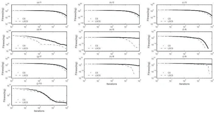
4.1.3 Test Group A: The Convergence Tests

Figure 1 presents the convergence progress of two algorithms (CS and LSCS) on a single run of 10000 iterations, and the dimension of nest (D) is 50. As for the results of the unimodal Problems, Fig. 1(from subfigure (a) to subfigure (d)) suggests that the LSCS algorithm with Converted learning module performs better than the standard algorithm in terms of search and converge capability. Especially, in solving Schwefels P2.22(Fig. 1-subfigure (d)), the performance of LSCS algorithm is particularly prominent. The results of the multimodal problems are presented in Fig. 1 (Fig. 1 or Fig. 1) (from sub-figure(e) to subfigure(j)) which suggests (suggest) a better reliability and a more desirable stability of LSCS over CS. Nevertheless, the result of the Rosebrock function(f10) shown in subfigure (j) of Fig. 1, after the last 10000 iterations, the convergence rate of the LSCS is lower

Table 2 The mean and SD of Test Group A

30D f₁ f₂ f₃

CS Mean 2.91E-16 3.18E-15 2.90E-13 SD 3.08E-16 3.45E-15 3.20E-13 LSCS Mean 3.47E-35 2.20E-34 2.26E-32 SD 5.82E-35 4.33E-34 5.57E-32

30D f₄ f₅ f₆

CS Mean 3.09E-07 1.08E-01 2.43E-07 SD 1.37E-07 4.68E-07 9.35E-07 LSCS Mean 3.51E-21 5.51E-15 7.38E-03 SD 3.90E-21 1.66E-15 8.56E-03

30D f₇ f₈ f₉

CS Mean 6.58E-13 4.79E+01 6.39E-01 SD 8.21E-13 7.99E+00 2.41E-01 LSCS Mean 5.35E-31 9.95E-02 0.00E+00

SD 7.78E-31 4.01E-01 0.00E+00

30D f₁₀

CS Mean 1.67E+01 SD 4.09E+00 LSCS Mean 3.22E+01 SD 2.94E+01

50D f1 f2 f3

CS Mean 2.65E-17 4.18E-16 4.35E-14 SD 2.34E-17 3.03E-16 2.72E-14 LSCS Mean 1.09E-27 2.44E-26 4.90E-25 SD 1.38E-27 3.87E-26 4.63E-25

50D f4 f5 f6

CS Mean 1.24E-08 6.79E-01 2.43E-07 SD 5.17E-09 2.22E+00 9.35E-07 LSCS Mean 4.48E-17 1.65E-14 2.13E-03 SD 2.90374E-17 5.94E-15 5.08E-03

50D f7 f8 f9

CS Mean 1.09E-11 8.05E+01 1.06E+00 SD 1.33E-11 9.73E+00 0.182 LSCS Mean 1.62E-22 5.18E+01 0.00E+00

SD 1.9817E-22 3.45E+01 0.00E+00

50D f10

CS Mean 4.60E+01 SD 1.98E+01 LSCS Mean 6.68E+01 SD 3.76E+01

than that of the standard CS. To find the optimal solution to the Rosebrock, the LSCS requires a certain number of iterations for the sake of particle diversity. In solving Ackley(f5), Griewangk(f6), Weierstrass(f8) and Rastrigin(f9) functions, the LSCS optimization algorithm quickly finds the global optimal solution(f(x) = 0), because the application of the Multi-Learning Strategies of the LSCS optimization algorithm has improved the searching capability of the nests.

4.2 Test Group B: The CEC2013 Test Suite

The previous analysis of Test Group A shows that the performance of the proposed LSCS is significantly better than that of the standard CS algorithm.In the following study, we use more complex benchmark functions (Group B: CEC2013 test suite) to examine the performance of the LSCS.The CEC2013 test suite consists of five Uni- modal functions(from f11 to f15), fifteen Basic Multimodal functions(from f16 to f30) and eight Compositions functions(from f31to f38), and they are more complex with rota- tion and displacement characteristics of the functions.

4.2.1 Test Group B: Experimental Setup

We compare the proposed algorithm LSCS with five ap- proaches, i.e., CS, TCPSO[26], SACS[10], CCS3[11]and

(5)

Fig. 1 Convergence performance of the CS and LSCS on Test Group A.

CLPSO[22].Comparative experiments are conducted within Test Group B. The functions of Test Group B are set at 30 and 50 respectively, and the iterations of the corresponding algorithm are set at 30000 and 50000 accordingly. The population of each algorithm is 40 and they run 30 times respectively. Parameter configurations of the comparing algorithms are listed below: 1) Standard CS: The probability switching parameter Pa = 0.25; 2) TCPSO:l = 2,w^M = 0.9,c^s₁ = c^s₂ = c₁^M = c^M₂ = c₃^M = 1.6; 3) SACS: The probability switching parameterPa =0.25; 4) CCS3: The probability switching parameter Pa = 0.25; 5) CLPSO:

w0 = 0.9,w1 = 0.4,c = 1.49445,Refreshing gap m = 7;

6) LSCS: The probability switching parameterPa = 0.25;

Refreshing gapm=7;

4.2.2 Performance Evaluation of Group B

The means and standard deviations of the algorithms on the CEC2013 test suite with 30D problems are shown in Table 3. The CCS3 algorithm and LSCS algorithm have demonstrated a better performance on five Unimodal functions (fromf11andf15).For f11andf15, the CCS3 and LSCS algorithms can find the optimal solution(0).Among the 15 basic multimodal functions, LSCS algorithm performs the best within 8 functions (namely, f16,f18,f19,f21,f23,f24, f25

and f27). Among the 8 compositions functions(from f31 to f₃₈),the LSCS algorithm has performed the best.Because the Elite Learning Perturbation Module prevents the bestnest from being trapped in the local optima, if the fitness of the bestnestis not improved formsuccessive fitness. And different the transition probabilityP_cvalues yield the best performance for diﬀerent 8 compositions functions. In order to compare the performance of the six algorithm,we also make

another set of experiments which is the CEC2013 test suite with 50D. According to the results of the 50D problems shown in Table 4, our proposed method LSCS still achieves the best or better performance against other comparing algorithms over most of the test functions.

4.2.3 Test Group B: The Non-Parametric Wilcoxons Rank Sum Test

Wilcoxons rank sum test returns p −Value and z. The p−Valuerepresents the minimal significance level for de- tecting diﬀerences.If thep−Valueis less than 0.05, it means that, the better result achieved by the best algorithm is sta- tistically significant in each case, and it is not obtained inci- dentally. Table 4 shows the non-parametric Wilcoxons rank sum test of the algorithms on the CEC2013 test suite with 30D problems. For the 30D problems, in function(s) f11

and f₁₅(Unimodal),function f₃₀(Multimodal) and functions f33, f36and f38(Composition), p−Valueobtained through Wilcoxons rank sum test are bigger than 0.05. About Uni- modal Functions(f11 and f15) and Composition Functions ( f₃₈), optimal solutions of the LSCS and CS are two inde- pendent samples, which have the same p−value,1.On the whole, in the CEC2013 test suite, LSCS achieves significant better performance against CS.

5. Conclusion

The global random walk of the standard CS algorithm is at the risk of excessive exploitation, and when it occurs nests lose the global exploration capacity and thus makes the algorithm prone to premature convergence. In this paper, we propose a cuckoo search algorithm with Multi-learning

(6)

Table 3 The result of CEC2013 functions with 30D, MaxFES:30000

Algo f₁₁ f₁₂ f₁₃ f₁₄ f₁₅ f₁₆ f₁₇

CS Mean 0.00E+00 4.87E+05 5.47E+05 3.05E+02 0.00E+00 4.45E-02 9.37E+01 SD 0.00E+00 1.27E+05 8.82E+05 5.57E+01 0.00E+00 5.82E-02 1.38E+01 TCPSO Mean 1.14E-12 2.65E+06 4.44E+08 1.87E+03 7.84E-13 3.33E+01 1.16E+02 SD 1.36E-12 1.45E+06 4.38E+08 8.02E+02 6.92E-13 2.18E+01 2.89E+01 SACS Mean 0.00E+00 3.46E+06 4.81E+07 1.36E+03 1.14E-13 1.32E+01 4.98E+01 SD 0.00E+00 1.21E+06 2.77E+07 3.45E+02 0.00E+00 4.01E+00 1.06E+01 CCS3 Mean 0.00E+00 3.85E+05 1.05E+05 2.83E+00 0.00E+00 3.65E-02 6.13E+01 SD 0.00E+00 1.43E+05 2.11E+05 2.59E+00 0.00E+00 3.83E-02 3.40E+01 CLPSO Mean 2.05E-13 6.11E+06 1.06E+08 5.55E+03 1.67E-13 1.50E+01 6.26E+01 SD 6.94E-14 1.78E+06 4.71E+07 1.19E+03 5.77E-14 4.18E+00 1.16E+01 LSCS Mean 0.00E+00 3.40E+05 8.05E+05 4.35E+04 0.00E+00 3.35E-04 6.59E+01 SD 0.00E+00 9.27E+05 1.61E+06 3.33E+04 0.00E+00 3.12E-04 2.48E+01

Algo f18 f19 f20 f21 f22 f23 f24

CS Mean 2.08E+01 2.80E+01 5.35E-04 8.95E-01 1.17E+02 1.56E+02 6.02E+02 SD 6.61E-02 1.92E+00 2.23E-03 3.04E-01 2.38E+01 3.10E+01 1.79E+02 TCPSO Mean 2.09E+01 2.73E+01 4.45E-01 8.34E+01 2.17E+02 2.29E+02 1.37E+03 SD 7.23E-02 3.11E+00 6.41E-01 2.49E+01 5.50E+01 2.57E+01 4.12E+02 SACS Mean 2.09E+01 2.76E+01 1.50E+00 0.00E+00 1.01E+02 1.36E+02 7.07E-01 SD 5.67E-02 2.05E+00 2.52E-01 0.00E+00 1.68E+01 1.39E+01 6.97E-01 CSS3 Mean 2.09E+01 2.42E+01 5.01E-03 0.00E+00 7.75E+01 1.20E+02 2.22E+02 SD 4.75E-02 1.94E+00 4.54E-03 0.00E+00 1.20E+01 1.67E+01 1.52E+02 CLPSO Mean 2.09E+01 2.25E+01 8.85E-01 1.25E-13 7.28E+01 1.23E+02 4.87E+02 SD 5.55E-02 1.72E+00 2.81E-01 9.49E-14 1.22E+01 2.23E+01 1.18E+02 LSCS Mean 2.07E+01 2.21E+01 6.45E-02 0.00E+00 8.90E+01 1.18E+02 1.81E-01 SD 9.88E-02 5.167398 4.02E-02 0.00E+00 2.99E+01 26.536110 5.05E-02

Algo f₂₅ f₂₆ f₂₇ f₂₈ f₂₉ f₃₀ f₃₁

CS Mean 4.03E+03 2.07E+00 5.63E+01 1.67E+02 4.79E+00 1.19E+01 2.04E+02 SD 2.75E+02 2.74E+00 7.28E+00 2.24E+01 5.73E-01 2.55E-01 4.62E+01 TCPSO Mean 5.38E+03 1.64E+00 9.93E+01 2.42E+02 8.09E+00 1.50E+01 3.34E+02 SD 1.13E+03 4.03E-01 2.17E+01 4.90E+01 3.12E+00 0.00E+00 1.02E+02 SACS Mean 3.64E+03 1.45E+00 3.04E+01 1.86E+02 2.31E+00 1.14E+01 2.50E+02 SD 2.53E+02 2.17E-01 7.42E-03 1.23E+01 3.17E-01 3.43E-01 4.95E+01 CSS3 Mean 3.81E+03 1.01E+00 3.89E+01 1.25E+02 3.31E+00 1.29E+01 2.33E+02 SD 3.00E+02 1.36E-01 3.43E+00 1.44E+01 6.38E-01 1.85E+00 4.79E+01 CLPSO Mean 3.18E+03 6.03E-01 3.21E+01 1.03E+02 7.64E-01 1.41E+01 1.62E+02 SD 3.12E+02 1.39E-01 3.10E+00 9.73E+00 2.51E-01 8.00E-01 4.76E+01 LSCS Mean 4.43E-01 1.74E+00 3.01E+01 1.36E+02 9.01E-01 1.21E+01 3.89E+02 SD 2.68E-01 5.77E-01 1.19E-01 3.41E+01 2.73E-01 9.22E-01 8.19E+01

Algo f32 f33 f34 f35 f36 f37 f38

CS Mean 8.42E+02 4.61E+03 2.78E+02 2.96E+02 2.00E+02 1.02E+03 3.00E+02 SD 2.62E+02 4.80E+02 4.97E+00 3.37E+00 7.07E-03 2.08E+02 0.00E+00 TCPSO Mean 1.55E+03 5.99E+03 2.70E+02 2.72E+02 3.30E+02 1.00E+03 5.19E+02 SD 4.69E+02 9.66E+02 9.82E+00 9.77E+00 7.34E+01 7.69E+01 5.62E+02 SACS Mean 1.76E+02 4.25E+03 2.68E+02 2.88E+02 2.00E+02 1.00E+03 3.00E+02 SD 2.95E+01 4.41E+02 8.34E+00 5.77E+00 4.93E-02 5.36E+01 0.00E+00 CCS3 Mean 2.82E+02 4.36E+03 2.44E+02 2.80E+02 2.00E+02 9.24E+02 2.93E+02 SD 1.11E+02 1.16E+03 5.37E+01 2.32E+01 5.53E-03 1.37E+03 3.65E+01 CLPSO Mean 4.30E+02 4.07E+03 2.38E+02 2.95E+02 1.97E+02 4.86E+02 1.61E+02 SD 8.54E+01 5.11E+02 2.79E+01 5.59E+00 1.02E+01 1.98E+02 8.74E+01 LSCS Mean 1.31E+02 4.40E+03 2.26E+02 2.77E+02 1.93E+02 7.92E+02 3.00E+02 SD 6.93E+01 8.00E+02 19.70212 1.19E+01 17.41992 1.48E+02 0.00E+00

strategies (LSCS). In LSCS, the converted learning module tries to make a coordinated cooperation between exploration and exploitation, and the Elite Learning Perturbation Mod- ule alleviates the premature convergence.

The Boundary Handling Approach adjusted by Gauss map overcomes the drawback of Set on Boundary. The proposed algorithm is evaluated on Test Group A(ten simple unimodal and multimodal functions) and Test Group B(the CEC2013 test suite). And it is compared with the standard CS and some other well-known existing optimization algorithms. The experimental results indicate that LSCS sub- stantially outperforms the standard CS algorithm in terms of convergence speed. Besides, LSCS can always find global optimal in the benchmark functions.

Future work may include the ability to add social learning to the nests of the LSCS algorithm, enabling information transfer between particles so as to find optimal solutions in complex environments. By using multi-population parti-

tioning, the nests of LSCS algorithm will be more hetero- geneous, so the exploration ability will be more desirable.

Nevertheless the more important question is how to apply the LSCS optimization algorithm in solving more complex optimization problems within the engineering domain.

Acknowledgments

This work is partially supported by the Anhui Province Phi- losophy and social sciences planning project under Grant No. AHSKZ2015D49, the University Humanities and social science Research Projects at the provincial level under Grant No. SK2018A0069,the Natural Science Foundation of the Educational Commission of Anhui Province of China under Grant No.KJ2018A0050, and the Key Research and Development Program of Anhui, China under Grant No.

201904a05020071.