Doctoral Thesis
A study on the density and sensitivity analysis concerning the
maximum of SDEs
Doctoral Program in Integrated Science and Engineering
Graduate School of Science and Engineering
concerning the maximum of SDEs
Tomonori Nakatsu
Department of Mathematical Science
Graduate School of Science and Engineering
In this thesis, we shall give some results on the existence of the den-sity function and sensitivity analysis concerning the maximum of some stochastic differential equations (SDEs, in short). The Malliavin calculus (or stochastic calculus of variations) plays an important role to obtain the results of this thesis.
In Chapter 1, we present the introduction of this thesis and the pre-liminary of Malliavin calculus.
In Chapter 2, we consider an m-dimensional SDE with coefficients which depend on the maximum of the solution. First, we prove the absolute continuity of the law of the solution. Then we prove that the joint law of the maximum of the ith component of the solution and the
i′th component of the solution is absolutely continuous with respect to the Lebesgue measure in a particular case.
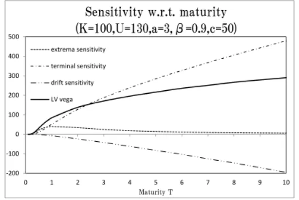
In Chapter 3, we give a decomposition formula to calculate the vega index (the sensitivity of an option contract with respect to changes in volatility) for options depending on the extrema (maximum or minimum) of a general one-dimensional model and study its behavior. Moreover, we compare the vega index obtained in this one-dimensional model with the one in the Black-Scholes model. Our mathematical and numerical results provide mainly three interesting properties of the vega index for barrier type options in the one-dimensional model: First, the vega index can be decomposed into three components which can be called extrema sensitivity, terminal (feature) sensitivity and drift sensitivity. Second, by using an example of up-in call options, we show that there is a barrier value at which the importance of extrema and terminal sensitivity are reversed. Third, extrema sensitivity is important only for options with short maturity as far as the vega index is concerned. The comparison of the vega index in two different models clarifies that the behavior of the vega index in the one-dimensional model considered in this thesis is far away from that in the Black-Scholes model. In the case of binary barrier options, each component of the decomposition formula for the vega index involves the Dirac delta functionals. Kernel methods are used in order to estimate the vega index in this setting.
I would like to express my deepest thanks to Professor Arturo Kohatsu-Higa, for his guidance and support from the summer of 2005 when we met for the first time. He has been taking care of me in terms of about studies and researches from our first encounter (even when I was a practitioner at a company). Needless to say, his constructive ideas and thoughtful comments largely contribute to this thesis.
I am also indebted to Professor Jirˆo Akahori who has supported my life at Ritsumeikan University. He has organized some symposiums dur-ing my doctoral course at which I have had the opportunities to give talks.
Professor Setsuro Fujiie has given me deep kindness throughout my PhD course.
Fruitful discussions with the following people: Professor Atsushi Takeuchi, Professor Masafumi Hayashi, Professor Masaaki Fukasawa and Song Xiaoming, improved this thesis. I would like to thank them.
I am thankful to Professor Taizo Chiyonobu, Professor Kazuhiro Yasuda, Professor Takahiro Aoyama, Professor Ngˆo Ho`ang Long and Professor Azmi Makhlouf for giving me encouragements to address my works.
I would like to thank the members the of weekly mathematical finance seminar: Professor Masatoshi Fujisaki, Professor Kenji Yasutomi, Pro-fessor Takuya Watanabe, Yuri Imamura, Nienlin Liu, Gˆo Yˆuki, Zhong Jie and Libo Li, for valuable talks.
I have received encouragements through talking with several practi-tioners and I must give my thanks to them.
My colleagues of Ristumeikan University: Hideyuki Tanaka, Hidemi Aihara and Takafumi Amaba, have given interesting and inspiring dis-cussions. I greatly appreciate them.
1 Introduction and preliminary 1
1.1 Problem of the existence of the density function . . . 1
1.2 Problem of the computation of Greeks . . . 1
1.3 Preliminary of Malliavin calculus . . . 2
2 Absolute continuity of the laws of a multi-dimensional stochastic differential equation with coefficients depending on the maximum 5 2.1 Introduction . . . 5
2.2 The existence, uniqueness and differentiability of the solution to (2.1) and the absolute continuity of the probability law of Xt . . . 6
2.3 The absolute continuity of the probability law of (Xti, Mti′) . . . 20
2.4 A concluding remark . . . 24
3 Volatility risk for options depending on extrema and its estimation using kernel methods 25 3.1 Introduction . . . 25
3.2 Main result: Vega index for options depending on the extrema . . . 27
3.3 Numerical experiment 1: Structure of the vega index . . . 33
3.3.1 Preliminary: assumptions of the one-dimensional model and the definition of the vega in the Black-Scholes model . . . 33
3.3.2 The case of payoff functions depending on only one component . . . 34
3.3.3 The case of payoff functions depending on the extrema and the terminal value of the underlying . . . 35
3.4 Kernel method . . . 38
3.5 Numerical experiment 2: Estimation of the vega index using the kernel method . . . 41
3.6 Conclusion and final remarks . . . 43
Appendix A . . . 44 Appendix A.1 . . . 44 Appendix A.2 . . . 45 Appendix A.3 . . . 46 Appendix A.4 . . . 46 Appendix A.5 . . . 49 Appendix B . . . 50 Appendix C . . . 51 vii
Appendix D . . . 53
Introduction and preliminary
1.1
Problem of the existence of the density function
In probability theory, we often consider an infinite-dimensional probability space, called the Wiener space. On the Wiener space, computing the expectation of a random variable implies integrating the random variable with respect to a probability measure defined on this infinite-dimensional space, called the Wiener measure. If we can prove the existence of the density function of the random variable, this integral with respect to the Wiener measure can be transformed to the integral with respect to the Lebesgue measure, namely, a measure on a finite-dimensional space.
Meanwhile, in mathematical finance, we often deal with options with non-smooth payoff functions (e.g. European call option or European put option). The price of options is defined by the expectation of random variables and the risks involved in options are defined by the sensitivities of the price of options with respect to market parameters. Thus, in order to compute these sensitivities, we are required to differentiate non-smooth payoff functions. The existence of the density function of the random variable guarantees that we can differentiate non-smooth payoff functions, as long as the Lebesgue measure of the set of all non-smooth points of the payoff functions is zero.
Therefore, to study the existence of the density function of random variables is one of the most important subject from a theoretical and a practical point of view.
Chapter 2 of this thesis is concerned with the problem of the existence of the density functions of an SDE whose coefficients are dependent on the maximum of the solution. One may interpret a result obtained in this chapter as an extension of a result in [7]. However, we shall give some results on the joint laws which are not considered in [7]. The results of Chapter 2 are taken from the published paper [15].
1.2
Problem of the computation of Greeks
In mathematical finance, the computation of the risks involved in options, called Greeks, is one of the most important problem since practitioners begin the hedging procedures for options based on the values of Greeks. There are some kinds of Greeks. For example, the sensitivity of option prices with respect to the current underlying asset’s price price is called the delta, and the sensitivity of the delta with respect to the current asset price is called the gamma. A market parameter which describes the variance of asset
prices is called the volatility, and the sensitivity with respect to the volatility is called the vega or vega index.
In the Black-Scholes model, the simplest financial model, the Greeks can be computed explicitly. However, in the other models which may perform better than the Black-Scholes model, the Greeks do not have the explicit formulas, therefore we are required to use some numerical techniques to compute the Greeks, such as the Monte Carlo simulation. Hence, the problem how we can express the Greeks is an interesting and important problem, mathematically and practically.
In practice, various types of options are traded by practitioners. A European option may be exercised only at the expiration date of the option (e.g. European call option or European put option). An option whose payoff is determined by the average underlying price over some pre-set period of time is called an Asian option. A lookback option is an option with the payoff depends on the maximum (or minimum) underlying asset’s price occurring over the life of the option. A barrier option is an option on the underlying asset whose price breaching the pre-set barrier level either springs the option into existence or extinguishes an already existing option.
In [6], the authors used the Malliavin calculus to calculate the Greeks for the first time. They obtained some expressions to compute the Greeks of some European options and Asian options, and showed that these expressions provide the better numerical results than ones obtained by a classical method, called the finite difference method. One can find a formula to compute the vega index for Asian options, in [1]. In [9], a method to compute the delta and gamma of lookback and barrier options is discussed and numerical results are also given.
In Chapter 3, we focus on the problem of the computations of the vega index for lookback and barrier options. We shall give an expression of the vega index, numerical results and a method to simulate the vega index for some specific options. The results of Chapter 3 are taken from the submitted paper [16].
1.3
Preliminary of Malliavin calculus
Recent advances of a differential calculus on the Wiener space, called the Malliavin calculus (or stochastic calculus of variations) provides many useful tools to us in order to try the problems mentioned in the previous subsections.
We introduce some basic tools of Malliavin calculus that will be used throughout the thesis. We refer to [17] to introduce Malliavin calculus. Let (Ω,F, P ) be the canonical Wiener space which supports a
d-dimensional Brownian morion W .
The class of real random variables of the form F = f (Wt1,· · · , Wtn), f ∈ Cb∞(R
nd;R), 0 ≤ t1,· · · , tn ≤ t is denoted by S. D1,p denotes a Banach space which is the completion of S with
re-spect to the norm
∥F ∥1,p= E[|F |p] 1 p + E ∫ t 0 d ∑ j=1 |Dj rF| 2dr p 2 1 p , where DjrF = n ∑ i=1 ∂f ∂xji(Wt1,· · · , Wtn)1[0,ti](r). 2
Dk,p is defined analogously, and its associated norm is denoted by ∥ · ∥k,p. Also, we define Dk,∞ = ∩p≥1Dk,pandD∞=∩p≥1∩k≥1Dk,p. For F, G∈ D1,2we define⟨DF, DG⟩H:=∫0t∑dj=1DrjF DjrGdr and ∥DF ∥2 H := ∫t 0 ∑d j=1|D j rF|2dr.
Now let us introduce a localization of Dk,p. Dk,p
loc denotes the set of random variables F such that
there exists a sequence{(Ωn, Fn), n≥ 1} ⊂ F × Dk,p with the following properties:
(i) Ωn↑ Ω, a.s.
(ii) F = Fn, a.s. on Ωn.
The following theorem is well-known and we shall use this theorem of obtain the results in Chapter 1.
Theorem 1. (Theorem 2.1.2 of [17]) Let F = (F1,· · · , Fm) be a random vector satisfying the following
conditions.
(i) Fi belongs to the spaceD1,p
loc, p > 1, for all i = 1,· · · , m.
(ii) The matrix γF := (⟨DFi, DFj⟩H)1≤i,j≤mis invertible a.s.
Then the law of F is absolute continuous with respect to the Lebesgue measure onRm.
Absolute continuity of the laws of a
multi-dimensional stochastic
differential equation with coefficients
depending on the maximum
2.1
Introduction
In this chapter, we deal with the following m-dimensional stochastic differential equation (SDE):
Xti= xi0+ d ∑ l=1 ∫ t 0 Ail(s, Xs, Ms)dWsl+ ∫ t 0 Bi(s, Xs, Ms)ds, 1≤ i ≤ m (2.1)
where W denotes a d-dimensional Brownian motion, Ai l, B
i: [0,∞) × R2m → R , 1 ≤ i ≤ m, 1 ≤ l ≤ d
are measurable functions and Ms = (Ms1,· · · , Msm) := (maxu≤sXs1,· · · , maxu≤sXsm). The purpose of
this chapter is to prove the absolute continuity of the joint law concerning the solution to (2.1) with Lipschitz continuous coefficients using Malliavin calculus. In [7], the authors proved that if m = d = 1,
A and B are H¨older continuous, for t > 0 the law of Xt is absolutely continuous with respect to the
Lebesgue measure on R, where Xt is a weak or strong solution to (2.1). The authors used the method
to analyze the characteristic function of Xt to prove the absolute continuity of the law of Xtin [7].
In this chapter, first we prove the absolute continuity of the law of Xt= (Xt1,· · · , Xtm) with respect
to the Lebesgue measure on Rm. Then we prove the absolute continuity of the law of (Mi t, Xi
′ t), 1 ≤ i, i′ ≤ m, with respect to the Lebesgue measure on R2 when Ai
l does not depend on the second space
variable. To analyze the law of (Mi t, Xi
′
t ) may be important in the field of applications such as finance.
Throughout this chapter, we use C or Ci, i ∈ N to denote a positive constant which may depend on
constants K, L, d, p, t and x0.
2.2
The existence, uniqueness and differentiability of the
solu-tion to (2.1) and the absolute continuity of the probability
law of X
tIn this section, firstly we prove the existence, uniqueness and differentiability of the solution to (2.1). Secondly we prove for t > 0, the absolute continuity of the probability law of Xtwhere X is the solution
to (2.1).
We assume the following:
(A1) There exist K, M, c > 0 such that
|A(t, x1, x2)− A(t, x′1, x′2)| + |B(t, x1, x2)− B(t, x′1, x′2)| ≤ K(|x1− x′1| + |x2− x′2|)
|A(t, x1, x2)| + |B(t, x1, x2)| ≤ L,
for any x1, x2, x′1, x′2∈ Rm and t≥ 0,
(A2) A(t, x1, x2) is continuous with respect to (t, x1, x2),
(A3) there exists c > 0 such that
|vTA(t, x
1, x2)|2≥ c|v|2,
for any v∈ Rm and x
1, x2∈ Rmand t≥ 0.
First, let us state a lemma on the existence of a unique solution to (2.1).
Lemma 1. Assume (A1), then (2.1) has a unique strong solution for any initial value x0 ∈ Rm.
Moreover we have E[|Mti|p]≤ C for any t ≥ 0, 1 ≤ i ≤ m and p ≥ 2. Proof. For s∈ [0, t] we define
Xs(0),i := xi Xs(n+1),i := x i + d ∑ l=1 ∫ s 0 Ail(u, X (n) u , M (n) u )dW l u+ ∫ s 0 Bi(u, Xu(n), M (n) u )du, 1≤ i ≤ m, n ≥ 0, (2.2) where Xu(n) := (X (n),1 u ,· · · , X (n),m u ) and M (n) u := (maxv≤uX (n),1 v ,· · · , maxv≤uX (n),m v ). From H¨older’s
inequality and Burkholder-Davis-Gundy’s inequality, it is easy to see that
E [ max u≤s Xu(n+1),i− Xu(n),i 2] ≤ C ( d ∑ l=1 E [∫ s 0 ( Ail(u, Xu(n), Mu(n))− Ail(u, Xu(n−1), Mu(n−1)) )2 du ] +E [∫ s 0 ( Bi(u, Xu(n), Mu(n))− Bi(u, Xu(n−1), Mu(n−1)) )2 du ]) 6
holds for s∈ [0, t] and 1 ≤ i ≤ m. By (A1) and a trivial inequality | maxv≤uXv(n),i−maxv≤uXv(n−1),i| ≤ maxv≤u|X (n),i v − X (n−1),i v |, we get E [ max u≤s Xu(n+1),i− Xu(n),i 2 ] ≤ CE [∫ s 0 ( |X(n) u − Xu(n−1)|2+|Mu(n)− Mu(n−1)|2 ) du ] ≤ C ∫ s 0 E [ m ∑ i=1 max v≤u |X (n),i v − X (n−1),i v | 2 ] du, therefore, E [m ∑ i=1 max u≤s|X (n+1),i u − X (n+1),i u | 2 ] ≤ C1 ∫ s 0 E [m ∑ i=1 max v≤u|X (n),i v − X (n−1),i v | 2 ] du, (2.3) for s∈ [0, t] and n ∈ N.
We define, for s∈ [0, t] and n ∈ N, f(n)(s) := E[∑m
i=1maxu≤s|X (n+1),i u − X (n+1),i u |2 ] , then we have f(n)(s)≤ C1n ∫ s 0 ∫ u1 0 · · · ∫ un−1 0 f(0)(un)dun· · · du1,
by (2.3). Now due to (A1), we obtain
f(0)(s) = E [ m ∑ i=1 max u≤s|X (1),i u − x0|2 ] ≤ C2,
for s∈ [0, t], thus we have
E [m ∑ i=1 max u≤s|X (n+1),i u − X (n),i u | 2 ] = f(n)(s)≤ (C1s) n n! C2. (2.4)
Relation (2.4) and the ˇCebyˇsev’s inequality give
P [m ∑ i=1 max s≤t |X (n+1),i s − X (n),i s | ≥ 1 2n+1 ] ≤ 2C2 (2C1t)n n! , (2.5)
for n ∈ N and the right hand side of (2.5) is a convergent series. From the Borel-Cantelli’s lemma, there exists ˜Ω ∈ F with P (˜Ω) = 1 such that for every ω ∈ ˜Ω there exists N(ω) ∈ N with ∑m
i=1maxs≤t|X
(k+1),i
s − Xs(k),i| < 2−(k+1) for k≥ N(ω). Moreover, this implies that m ∑ i=1 max s≤t |X (k+m′),i s − X (k),i s | ≤ 2−k, (2.6)
for every m′ ∈ N, k ≥ N(ω). We see then that the sequence of sample paths {Xs(n), s ∈ [0, t]} is
convergent in the supremum norm on continuous functions, which concludes the existence of a continuous limit{Xs, s∈ [0, t]} for all ω ∈ ˜Ω.
Now let us prove that {Xs, s∈ [0, t]} satisfies (2.1). Firstly, we shall consider the Lebesgue integral part. Due to (A1), we have for s∈ [0, t]
∫ s 0 Bi(u, Xu(n), Mu(n))du− ∫ s 0 Bi(u, Xu, Mu)du 2 ≤ C ∫ s 0 |M(n) u − Mu| 2du,
and (2.6) gives that maxu≤s|Xui − X
(n),i
u | ≤ 2−nfor n≥ N(ω). Thus, we get that
∫0sBi(u, Xu(n), Mu(n))du− ∫ s 0 Bi(u, Xu, Mu)du 2→ 0, holds as n→ ∞, a.s.
Next, we shall consider the stochastic integral part. We observe from (2.4) that for fixed u∈ [0, t], the sequence of random variables{Mu(n),i}n∈N is a Cauchy sequence in L2(Ω,F, P ). Indeed, from (2.4)
we get E [ |M(n),i u − M(n ′),i u |2 ] ≤ E [ max v≤u|X (n),i v − X(n ′),i v | ] ≤ n−1 ∑ j=n′ E [ max v≤u|X (j+1),i v − X (j),i v | 2 ] → 0,
as n, n′ → ∞. Therefore, there exists ˜Mui such that M
(n),i
u → ˜Mui in L2(Ω,F, P ). Since M
(n),i
u → Mui,
a.s., we have E[|Mu− ˜i Mu|] ≤ lim infni
→∞E[|Mu(n),i− ˜Mu|] = 0 and this implies that E[|Mu(n),i−Mu|i 2]→ 0
as n→ ∞. From (A1), we have for s ∈ [0, t]
E [ d ∑ l=1 ∫ s 0 ( Ail(u, Xu(n), Mu(n))− Ail(u, Xu, Mu) ) dWul 2] ≤ C ∫ s 0 E [ |M(n) u − Mu| 2]du. (2.7)
By (A1), we have E[|Mu(n),i|2]≤ C3and Fatou’s lemma gives E[|Mu|i 2]≤ lim infn→∞E[|M (n),i
u |2]≤ C3.
From (2.7) and the bounded convergence theorem, we have
E [ d ∑ l=1 ∫ s 0 ( Ail(u, Xu(n), Mu(n))− Ail(u, Xu, Mu) ) dWul 2] → 0,
as n→ ∞, thus, by taking a subsequence one has
∑d l=1 ∫ s 0 ( Ail(u, Xu(n), Mu(n))− Ail(u, Xu, Mu) ) dWul 2 → 0, (2.8)
as n→ ∞, a.s. Therefore, for t > 0, {Xs, s∈ [0, t]} satisfies (2.1).
Next, we shall prove the pathwise uniqueness of the equation (2.1). We assume that for fixed t > 0,
{Xs, s∈ [0, t]} and { ˇXs, s∈ [0, t]} satisfy (2.1). From (A1), it is easy to see that E [ max u≤s |X i u− ˇX i u|2 ] ≤ C ∫ s 0 E [m ∑ i=1 max u≤v |X i u− ˇX i v|2 ] dv,
thus, E [m ∑ i=1 max u≤s|X i u− ˇX i u|2 ] ≤ C ∫ s 0 E [m ∑ i=1 max u≤v |X i u− ˇX i v|2 ] dv
holds, then by defining g(s) := E[∑mi=1maxu≤s|Xui − ˇXu|i 2
]
and applying the Gronwall’s lemma to g(s), we have E[∑mi=1maxu≤s|Xui − ˇXu|i 2
]
= 0 for s∈ [0, t]. Therefore, one has the pathwise uniqueness of the solution{Xs, s∈ [0, t]} to (2.1) for fixed t > 0 by the continuity of {Xs, s∈ [0, t]}.
Since t > 0 is arbitrary, we have the existence of a unique strong solution{Xs, s∈ [0, ∞)} to (2.1). Moreover, E[|Mi
t|p]≤ C for p ≥ 2 is a consequence of (A1).
Now, let us prove the property of the time when one-dimensional process {Xsi, s∈ [0, t]} attains its
maximum on [0, t]. This property plays an important role to prove the absolute continuity of the joint law of (Mti, Xi
′ t).
Lemma 2. Under (A1)-(A3), for any t≥ 0 and 1 ≤ i ≤ m, {Xsi, s∈ [0, t]} attains its maximum on
[0, t] on a unique point τti and 0 < τti< t, a.s.
Proof. We define a new probability measure ˜P by
d ˜P dP := exp [ − d ∑ l=1 ∫ t 0 Cl(s, Xs, Ms)dWsl ] ,
where for x1, x2 ∈ Rm and s > 0, d-dimensional vector C(s, x1, x2) is defined by C(s, xs, x2) :=
[AT(AAT)−1B](s, x1, x2). Define a d-dimensional process ˜W by
˜
Ws:= Wsl+ ∫ s
0
Cl(u, XuMu), 1≤ l ≤ d.
Then by the Girsanov’s theorem,{ ˜Ws, s∈ [0, t]} is a d-dimensional Brownian motion under ˜P , therefore {Xs, s∈ [0, t]} can be expressed as Xsi= xi0+ d ∑ l=1 ∫ s 0 Ail(u, Xu, Mu)d ˜Wul, 1≤ i ≤ m, (2.9)
and for each 1≤ i ≤ m, {Xi
s, s∈ [0, t]} is a martingale by (A1). Let {Fs, s∈ [0, t]} be the augmentation
of the Brownian filtration generated by { ˜Ws, s∈ [0, t]}. For s ∈ [0, t], we define T (s) := inf{t > 0 : ⟨Xi⟩t> s} then the time-changed process
Bs:= XT (s)i ,Gs:=FT (s), s∈ [0, t]
is a standard one-dimensional Brownian motion. Moreover, by (A3),{Xi
s, s∈ [0, t]} can be written as Xsi= xi0+ B⟨Xi⟩s
First, let us prove that ˜ P ( max s≤t X i s= x i 0 ) = 0. By the law of iterated logarithm for Brownian motion, we have
lim sup s↓0 Xi s− xi0 √ 2⟨Xi⟩slog log( 1 ⟨Xi⟩s ) = lim sups↓0 √ B⟨Xi⟩s 2⟨Xi⟩slog log( 1 ⟨Xi⟩s ) = 1, ˜ P -a.s., thus ˜ P ( max s≤t X i s= x i 0 ) ≤ ˜P(Xsi≤ xi0,∀s ∈ [0, t])= 0. Then, we shall prove that
˜ P ( max s≤t X i s= Xti ) = 0.
We note that for t > 0,⟨Xi⟩t is a stopping time for the filtrationGs, since {⟨Xi⟩t≤ s} = {T (s) ≥ t} ∈ FT (s)=Gs. We define ˇ Bs:= { Bs, s∈ [0, t] Bt+ ˆWs− ˆWt, s∈ (t, ∞) (2.10)
and ˇFs:= σ(Bu, u≤ s) ∨ σ( ˜Wu, u≤ s), where { ˆWs, s∈ [0, ∞)} is a one-dimensional Brownian motion
independent of B, then we find that{ ˇBs, s∈ [0, ∞)} is a one-dimensional Brownian motion, since we can
easily check that{ ˇBs, s∈ [0, ∞)} is a ˇFs-martingale and its quadratic variation is given by{s, s ∈ [0, ∞)}. Let{B′s, s∈ [0, ∞)} be a one-dimensional Brownian motion independent of { ˇBs, s∈ [0, ∞)}. Define
ˆ
Bs:=
{ ˇ
Bs, s∈ [0, ∞)
B−s′ , s∈ (−∞, 0) (2.11)
then { ˆBs, s∈ (−∞, ∞)} is a two sided Brownian motion. By the definition of ˇFs, ⟨Xi⟩t is a stopping
time for the filtration ˇFs, therefore from Exercise 2.4 of [14], { ˆB⟨Xi⟩t−s− ˆB⟨Xi⟩t, s∈ [0, ∞)} is a
one-dimensional Brownian motion. Again, by the law of iterated logarithm for Brownian motion, we have
−1 = lim inf s↓0 ˆ B⟨Xi⟩t− ˆB⟨Xi⟩t−s √ 2s log log(1s) = lim inf s↓0 ˆ B⟨Xi⟩t− ˆB⟨Xi⟩t−s √ 2(⟨Xi⟩t− ⟨Xi⟩t −s) log log ( 1 ⟨Xi⟩t−⟨Xi⟩t−s ) = lim inf s↓0 B⟨Xi⟩t− B⟨Xi⟩t −s √ 2(⟨Xi⟩t− ⟨Xi⟩t −s) log log ( 1 ⟨Xi⟩t−⟨Xi⟩t −s ) = lim inf s↓0 Xi t− Xti−s √ 2(⟨Xi⟩t− ⟨Xi⟩t −s) log log ( 1 ⟨Xi⟩t−⟨Xi⟩t−s ),
˜ P -a.s. Therefore, ˜ P ( max s≤t X i s= X i t ) ≤ ˜P(Xsi≤ Xti,∀s ∈ [0, t])= 0. Finally, let us prove the uniqueness of τi
t on [0, t]. As mentioned before, we can write Xsi= xi0+ B⟨Xi⟩s for s∈ [0, t]. Define ¯ θt := sup { s≤ t : B⟨Xi⟩ s = sup 0≤u≤t B⟨Xi⟩ u } , θt := inf { s≤ t : B⟨Xi⟩s= sup 0≤u≤t B⟨Xi⟩u } , and ¯ τt := sup { s≤ t : Bs= sup 0≤u≤t Bu } , τt := inf { s≤ t : Bs= sup 0≤u≤t Bu } .
Then by the definitions, we have ¯
θt=⟨Xi⟩−1τ¯
⟨Xi⟩t, θt=⟨X
i⟩−1 τ⟨Xi⟩t.
Thus, one has ˜ P(θt< ¯θt< t ) = P˜ ( τ⟨Xi⟩ t < ¯τ⟨Xi⟩t<⟨X i⟩t) = P˜ ∪ r1,r2∈Q r1<r2 { τ⟨Xi⟩t < r1< ¯τ⟨Xi⟩ t < r2<⟨X i⟩t} = ∑ r1,r2∈Q r1<r2 ˜ P ( τ⟨Xi⟩t < r1< ¯τ⟨Xi⟩t < r2<⟨Xi⟩t ) ,
whereQ denotes the set of all rational numbers. On {τ⟨Xi⟩t < r1< ¯τ⟨Xi⟩t < r2<⟨Xi⟩t}, the definition
of ¯τ shows ¯ τ⟨Xi⟩ t = sup { s≤ r2: Bs= sup 0≤u≤r2 Bu } , (2.12)
and the definition of τ shows
τ⟨Xi⟩t = inf { s≤ r1: Bs= sup 0≤u≤r1 Bu } . (2.13)
Since Bτ¯⟨Xi⟩t = Bτ⟨Xi⟩t holds ˜P -a.s., (2.12) and (2.13) imply that sup 0≤u≤r1 Bu= sup 0≤u≤r2 Bu
holds ˜P - a.s. Therefore, we have
˜ P ( τ⟨Xi⟩ t < r1< ¯τ⟨Xi⟩t< r2<⟨X i⟩t) ≤ ˜P ( ¯ τ⟨Xi⟩t ∈ (r1, r2), sup 0≤u≤r1 Bu= sup 0≤u≤r2 Bu ) = P˜ ( sup { s≤ r2: Bs= sup 0≤u≤r2 Bu } ∈ (r1, r2), sup 0≤u≤r1 Bu= sup 0≤u≤r2 Bu ) = 0, where the last equality follows from Proposition 4 in Section VI of [2]. This finishes the proof.
Let us prove a lemma on the differentiability of the maximum of a continuous process which is similar to Proposition 2.1.10 of [17]
Lemma 3. For t≥ 0, let { ˆXs, s∈ [0, t]} be a one-dimensional continuous process. Suppose that
(i) E[sups≤t| ˆXs|2] <∞,
(ii) for any s∈ [0, t], ˆXs∈ D1,2 and E[sups≤t∥D ˆXt∥2H] <∞. Then ˆMt= sups≤tXsˆ ∈ D1,2 and we have
E [ ∥D ˆMt∥2 H ] ≤ E [ sup s≤t ∥D ˆXs∥2 H ] . (2.14)
Moreover, if we assume that
(iii) { ˆXs, s∈ [0, t]} attains its maximum on a unique point ˆτt∗,
(iv) for 1≤ j ≤ d, and almost every r, {Dj
rXs, sˆ ∈ [0, t]} is continuous except for s = r, and
(v) for 1≤ j ≤ d, E[∫0tsupr≤s≤t|DjrXs|ˆ 2dr] <∞, then we have
DjrMtˆ = DrXˆτˆt∗, a.e.r, (2.15)
where we have defined DrXˆτˆt∗ := DrXs|s=ˆˆ τt∗.
Proof. Let{tk}k≥0 be a dense subset of [0, t] and define ˆ Mtn := max{ ˆXt1,· · · , ˆXtn}. Define A1:={ ˆXt1 = ˆM n t}, Ak :={ ˆXt1 ̸= ˆM n t,· · · , ˆXtk−1 ̸= ˆM n t, ˆXtk= ˆM n t}, 2 ≤ k ≤ n.
Then, by the local property of operator D we have D ˆMtn = n ∑ k=1 1AkD ˆXtk.
By Proposition 2.1.10 of [17], Mtˆ = sup0≤s≤tXsˆ belongs to D1,2 and D ˆMn
t → D ˆMt(n → ∞) in
the weak topology of L2(Ω; L2([0, t];Rd)) under (i) and (ii). We obtain (2.14) from E[∥D ˆMt∥2
H] ≤
lim infn→∞E[∥D ˆMtn∥2H].
Let us prove (2.15). For ω∈ Ak we define ˆτn∗:= tk. Then ˆτn∗→ ˆτt∗, a.s. due to (iii), and we have
D ˆMtn=
n
∑
k=1
1AkD ˆXτˆn∗ = D ˆXτˆn∗,
where we have defined D ˆXˆτn∗ := D ˆXs|s=ˆτn∗. Note that, if r = ˆτn∗, then D ˆXˆτn∗ is not well defined, due to
the discontinuity; thus the rigorous meaning of the above equality is that DrMˆtn = DrXˆˆτn∗ for almost
every r with probability 1. Now let us prove
E ∫ t 0 d ∑ j=1 DrjXˆτˆn∗ujrdr → E ∫ t 0 d ∑ j=1 DjrXˆτˆt∗ujrdr , (2.16)
for any u∈ L2(Ω; L2([0, t];Rd)). We have
E ∫ t 0 d ∑ j=1 DrjXˆτˆn∗ujrdr − E ∫ t 0 d ∑ j=1 DjrXˆτˆt∗ujrdr = E ∫ t 0 d ∑ j=1 (DrjXˆˆτn∗ − DrjXˆτˆt∗)ujrdr . (2.17) From (iv), we have Dj
rXˆτˆn∗ → DrjXˆˆτt∗ for r ̸= ˆτt∗ then DrjXˆτˆn∗ → DjrXˆτˆt∗, for almost every r with
probability 1. As|Dj
rXˆτˆn∗− DjrXˆτˆt∗|2≤ 2 sup0≤s≤t|DrjXs|ˆ 2 and (v), we have
∫ t 0 d ∑ j=1 |Dj rXˆτˆn∗− DjrXˆˆτt∗|2dr→ 0 (n → ∞), a.s. Due to E[|Dj
rXˆτˆn∗− DjrXˆˆτt∗|2]≤ 2E[sup0≤s≤t|DjrXˆs|2] and (v), we have
lim n→∞E ∫ t 0 d ∑ j=1 |Dj rXˆˆτn∗ − DrjXˆτˆt∗|2 dr = 0. Then we obtain (2.16). Since D ˆMn
t converges to D ˆMt weakly in L2(Ω; L2([0, t];Rd)) and (2.16) holds,
we have E ∫ t 0 d ∑ j=1 ( DjrXˆˆτt∗ − DrjMˆt ) ujrdr = 0,
for any u ∈ L2(Ω; L2([0, t];Rd)). By the fact that ˆMt belongs to D1,2 and (v), we have {DrXˆτˆt∗ −
DrMt, rˆ ∈ [0, t]} ∈ L2(Ω; L2([0, t];Rd)). Therefore we have (2.15) with taking ur= DrXˆτˆt∗− DrMtˆ and
this finishes the proof.
Remark 1. In Lemma 3, if we assume that { ˆXs, s∈ [0, t]} is adapted, then we have DrXˆτˆt∗ = 0 for
almost every r such that r > ˆτt∗. Thus, in this case, we can write DrMtˆ = 1[0,ˆτt∗)(r)DrXˆτˆt∗, for almost
every r.
Next, let us prove the differentiability of the solution to (2.1) in Malliavin sense.
Lemma 4. Assume (A1)-(A3). Then, for s∈ [0, t] and 1 ≤ i ≤ m, Xi
s, Msi belong toD1,2. Moreover, {Dj
rXsi, s∈ [r, t]} satisfies the following equation:
DrjXsi = Aij(r, Xr, Mr) + ∫ s r ( ¯Aik,l(u)DjrXuk+ ˜Aik,l(u)DrjMuk)dWul + ∫ t r
( ¯Bik(u)DjrXuk+ ˜Bki(u)DjrMuk)du (2.18)
for r≤ s, a.e., and
DirXsi= 0, (2.19)
for r > s, a.e., where ¯Ak,l(u), ˜Ak,l(u), ¯Bk(u) and ˜Bk(u) are uniformly bounded and adapted m-dimensional processes.
Proof. We will use the Picard approximation from Lemma 1, so Xs(n), M
(n)
s are the processes
con-structed by recurrence there. The proof of this lemma uses the proof of Theorem 2.2.1 of [17]. We need to extend the proof to equation with coefficients which depend on the maximum process. We start by proving Xs(n),i ∈ D1,2 for s ∈ [0, t], 1 ≤ i ≤ m and n ≥ 0. If we assume X
(n),i
s ∈ D1,2 and
E[∫0ssupu≤v∥DX
(n),i
u ∥2Hdv] <∞ for s ∈ [0, t] then we have M
(n),i
s ∈ D1,2 for s∈ [0, t] by Lemma 3 and
E [∫ t 0 ∫ t 0 |Dj r(A i l(u, X (n) u , M (n) u ))| 2drdu ] ≤ C (m ∑ k=1 E [∫ t 0 ∫ t 0 |Dj rX (n),k u | 2drdu ] + 2m ∑ k=m+1 E [∫ t 0 ∫ t 0 |Dj rM (n),k u | 2drdu ]) = C (m ∑ k=1 ∫ t 0 E [∫ u 0 |Dj rX (n),k u | 2dr ] du + 2m ∑ k=m+1 ∫ t 0 E [∫ u 0 |Dj rM (n),k u | 2dr ] du ) ≤ C ∑m k=1 ∫ t 0 E ∫ u 0 d ∑ j=1 |Dj rX (n),k u | 2dr du + ∑2m k=m+1 ∫ t 0 E ∫ u 0 d ∑ j=1 |Dj rM (n),k u | 2dr du = C (m ∑ k=1 E [∫ t 0 sup u≤s∥DX (n),k u ∥ 2 Hds ] + m ∑ k=1 E [∫ t 0 sup u≤s∥DM (n),k u ∥ 2 Hds ]) ≤ C m ∑ k=1 E [∫ t 0 sup u≤s∥DX (n),k u ∥2Hds ] <∞ (2.20)
by (2.14). Therefore, from Proposition 1.3.8 of [17], we have for s∈ [0, t], Xs(n+1),i∈ D1,2 and DrjXs(n+1),i = Aij(r, Xr(n), Mr(n)) + ∫ s r [ ¯
A(n),ik,l (u)DjrXu(n),k+ ˜A(n),ik,l (u)DrjMu(n),k
] dWul + ∫ t r [ ¯
B(n),ik (u)DrjXu(n),k+ ˜B(n),ik (u)DrjMu(n),k
]
du,
where ¯A(n)k,l, ˜A(n)k,l, ¯Bk(n)and ˜Bk(n) are uniformly bounded and adapted m-dimensional processes. Now, by
(A1) and (2.14), one has
E sup u≤s d ∑ j=1 ∫ u 0 ∑d l=1 m ∑ k=1 ∫ u r [ ¯ A(n),ik,l (v)DjrXv(n),k+ ˜A(n),ik,l (v)DrjMv(n),k ] dWvl 2 dr ≤ E sup u≤s d ∑ j=1 ∫ u 0 sup u≤s ∑d l=1 m ∑ k=1 ∫ u r [ ¯ A(n),ik,l (v)DrjXv(n),k+ ˜A(n),ik,l (v)DjrMv(n),k ] dWvl 2 dr = d ∑ j=1 ∫ s 0 E [ sup u≤s ∑d l=1 m ∑ k=1 ∫ u r [ ¯ A(n),ik,l (v)DjrXv(n),k+ ˜A (n),i k,l (v)D j rMv(n),k ] dWvl 2 ] dr ≤ C d ∑ j=1 ∫ s 0 E [ d ∑ l=1 ∫ s r ∑m k=1 [ ¯ A(n),ik,l (v)DjrXv(n),k+ ˜A(n),ik,l (v)DjrMv(n),k ] dv 2] dr ≤ C d ∑ j=1 ∫ s 0 E [ d ∑ l=1 ∫ s r m ∑ k=1 ( |Dj rX (n),k v | 2+|Dj rM (n),k v | 2)dv ] dr = C d ∑ j=1 ∫ s 0 E [ d ∑ l=1 ∫ s 0 m ∑ k=1 ( |Dj rX (n),k v | 2+|Dj rM (n),k v | 2)dv ] dr = C d ∑ j=1 ∫ s 0 E [ d ∑ l=1 ∫ s 0 m ∑ k=1 ( |Dj rX (n),k v | 2+|Dj rM (n),k v | 2)dr ] dv = C d ∑ j=1 ∫ s 0 E [ d ∑ l=1 ∫ v 0 m ∑ k=1 ( |Dj rX (n),k v | 2+|Dj rM (n),k v | 2)dr ] dv = C m ∑ k=1 ∫ s 0 E [ ∥DX(n),k v ∥ 2 H+∥DM (n),k v ∥ 2 H ] ≤ C m ∑ k=1 ∫ s 0 E [ sup u≤v ∥DX(n),k u ∥ 2 ] dv,
and the same computation as the above gives
E [ sup u≤s ∫ u 0 ∑m k=1 ∫ s r [ ¯ Bk(n),i(v)DjrXv(n),k+ ˜B(n),ik (v)DrjMv(n),k ] dv 2 dr ] ≤ C m ∑ k=1 ∫ s 0 E [ sup u≤v ∥DX(n),k u ∥ 2 ] dv. Thus, we have m ∑ i=1 E [ sup u≤s ∥DX(n+1),i u ∥ 2 H ] ≤ C1+ C2 ∫ s 0 m ∑ i=1 E [ sup u≤v ∥DX(n),i u ∥ 2 H ] dv, (2.21)
and this implies Ms(n+1),i∈ D1,2 and E[
∫s
0 supu≤v∥DX
(n+1),i
u ∥2Hdv] <∞ for s ∈ [0, t] by Lemma 3.
Due to (2.21) and Lemma 3, we have supnE[∥DXs(n),i∥2H] < ∞ and supnE[∥DM
(n),i
s ∥2H] ≤
supnE[supu≤s∥DXu(n),i∥] < ∞. By the fact that Xs(n),i → Xsi, M
(n),i
s → Msi in L2(Ω) and Lemma
1.2.3 of [17], Xi
s and Msi belong toD1,2 for s∈ [0, t]. Moreover DX
(n),i
s and DM
(n),i
s converge to DXsi
and DMi
s in the weak topology of L2(Ω; L2([0, t];Rd)).
Let us prove (2.18). We have
E [∫ t 0 ∫ t 0 |Dj r(A i l(u, Xu, Mu))| 2drdu ] ≤ C m ∑ k=1 ∫ t 0 E[∥DXuk∥2H+∥DMuk∥2H]du <∞
by the same calculation as (2.20), the fact that E[∥DMk
u∥2H] ≤ lim infn→∞E[∥DM
(n),k
u ∥2H] ≤
lim infn→∞E[supv≤u∥DX
(n),k
v ∥2H] holds and (2.21). Therefore, we have (2.18) and the proof is
com-pleted.
Lemma 5. Assume (A1)-(A3). Then, for {Xsi, s∈ [0, t]} and p ≥ 2 we have E [∫ s 0 sup r≤u≤s |DjXu|i pdr ] <∞, (2.22)
and assumptions (i)-(v) of Lemma 3 hold. Moreover, for s∈ [0, t] and p ≥ 2, Xi
s, Msi∈ D1,p. Proof. First, let us prove (2.22) for p = 2. We have
d ∑ j=1 E [∫ s 0 sup r≤u≤s|D j rXu|i 2dr ] ≤ C1+ C2 (∫ s 0 E [ sup r≤u≤s ∫ru∑d l=1 ( ¯ Aik,l(v)DrjXvk+ ˜Aik,l(v)DjrMvk ) dWvl 2] dr + ∫ s 0 E [ sup r≤u≤s ∫ru(B¯i k(v)D j rX k v+ ˜B i k(v)D j rM k v ) dv 2] dr ) ≤ C1+ C2 (∫ s 0 E [ d ∑ l=1 ∫ s r ( ¯ Aik,l(v)DjrXvk+ ˜Aik,l(v)DrjMvk )2 dv ] dr + ∫ s 0 E [∫ s r ( ¯ Bki(v)DjrXvk+ ˜Bki(v)DrjMvk )2 dv ] dr ) ≤ C1+ C2 ∫ s 0 E [∫ s r m ∑ k=1 ( ∥Dj rX k v∥ 2+∥Dj rM k v∥ 2)dv ] dr = C1+ C2E [∫ s 0 ∫ s 0 m ∑ k=1 ( ∥Dj rX k v∥ 2+∥Dj rM k v∥ 2)drdv ] = C1+ C2 ∫ s 0 E [∫ v 0 m ∑ k=1 ( ∥Dj rX k v∥ 2+∥Dj rM k v∥ 2)dr ] dv = C1+ C2 m ∑ k=1 ∫ s 0 E[∥DXvk∥2H+∥DMvk∥2H ] dv <∞, (2.23)
by the fact that E[∥DMk
v∥2H] ≤ lim infn→∞E[∥DM
(n),k
v ∥2H] ≤ lim infn→∞E[supu≤v∥DX
(n),k
u ∥2H] is
true, (2.18) and (2.21). This implies that (v) holds for Xi. (i) follows from Lemma 1 and we have (ii) by (2.22) for p = 2. (iii) holds due to Lemma 2 and we have (iv) by (2.18) and (2.19).
Let us prove (2.22) for p > 2. It suffices to prove
E ∫ t 0 m ∑ i=1 d ∑ j=1 sup r≤s≤t |Dj rX i s|pdr ≤ C1+ C2 ∫ t 0 E ∫ u 0 m ∑ i=1 d ∑ j=1 sup r≤s≤u |Dj rX i s|pdr du. (2.24)
However, we get (2.24) from the same computation as (2.23) and an inequality
∥DMk u∥ p H≤ C d ∑ j=1 ∫ u 0 sup r≤s≤u|D j rX k u|pdr,
which follows from (2.18), (2.19) and (2.15). From (2.22) we have Xi
s, Msi ∈ D1,p for s ∈ [0, t] and p≥ 2.
Now we consider two m× m matrix-valued process defined by
Yji(s) = δji+ ∫ s 0 ¯ Aik,l(u)Yjk(u)dWul+ ∫ s 0 ¯ Bki(u)Yjk(u)du , 1≤ i, j ≤ m (2.25) and Zji(s) = δji− ∫ s 0 Zki(u) ¯Akj,l(u)dWul− ∫ s 0
Zki(u)[ ¯Bkj(u)− ¯Akα,l(u) ¯Aαj,l(u)]du, 1≤ i, j ≤ m. (2.26) By the argument in section 2.3 of [17], we have Y−1(s) = Z(s). Let us express Dj
rXsi by using Y (s) and Z(s).
Lemma 6. For s∈ [r, t] and 1 ≤ i ≤ m, 1 ≤ j ≤ d, DjXi
ssatisfies DrjXsi = Yki(s)Zkk′(r)Ak ′ j (r) + Y i k(s) ∫ s r Zkk′(u) ˜Ak ′ l′,l(u)D j rM l′ udW l u +Yki(s) ∫ s r Zkk′(u)[ ˜Bk ′ l′(u)− ¯A k′ α,lA˜ α l′,l(u)]D j rM l′ udu. (2.27)
Proof. From (2.18), (2.25), (2.26) and Itˆo’s formula, one has for 1≤ i ≤ m and 1 ≤ j ≤ d,
m ∑ k′=1 Zki′(s)DrjX k′ s = m ∑ k′=1 Zki′(r)Ak ′ j (r, Xr, Mr) + m ∑ k′=1 ∫ s r Zki′(u)d(DjrX k′ u ) + m ∑ k′=1 ∫ s r DrjXuk′dZki′(u) + m ∑ k′=1 ∫ s r d⟨Zki′(·), DrjX k′ · ⟩u = Zki′(r)Ak ′ j (r, Xr, Mr) + ∫ s r Zki′(u) ¯Ak ′ l′,l(u)D j rM l′dWl u + ∫ s r Zki′(u)[ ˜Bk ′ l′ (u)− ¯A k′ α,l(u) ˜A α l′,l(u)]D j rM l′ udu.
By the definition of (2.25) and (2.26), we have DrjXsi= m ∑ k,k′=1 Yki(s)Zkk′(s)DjXk ′ s ,
therefore, the result follows.
Now we prove the absolute continuity of the law of Xtwhich is the main theorem of this section.
Theorem 2. Assume (A1)-(A3), then for t > 0, Xthas the absolutely continuous probability law with respect to the Lebesgue measure onRm.
Proof. Let us prove∫0t|vTDrXt|2dr > 0 for nonzero vector v ∈ Rm. By (2.27) and a trivial inequality (a + b)2≥ a22 − b2, a, b∈ R, we have |vTDrXt|2 ≥ 1 2 d ∑ j=1 ∑m i=1 viYki(t)Z k k′(r)A k′ j (r) 2 − d ∑ j=1 ∑m i=1 viYki(t) (∫ t r Zkk′(s) ˜Ak ′ l′,l(s)D j rM l′ sdW l s+ ∫ t r Zkk′(s)[ ˜Bk ′ l′ (s)− ¯A k′ α,lA˜ α l′,l(s)]D j rM l′ sds ) 2 =: 1 2 d ∑ j=1 ∑m i=1 viYki(t)Z k k′(r)A k′ j (r) 2+ Ar,t. Then we have E [ 1 ε ∫ t t−ε Ar,tdr ] ≤ 1 εE ∫ t t−ε d ∑ j=1 ∑m i=1 viYki(t) (∫ t r Zkk′(s) ˜Ak ′ l′,l(s)D j rM l′ sdW l s + ∫ t r Zkk′(s)[ ˜Bk ′ l′(s)− ¯Ak ′ α,lA˜αl′,l(s)]DrjMl ′ sds ) 2dr ] ≤ C ε d ∑ j=1 m ∑ i=1 |vi|2E [∫ t t−ε Yi k(t) (∫ t r Zkk′(s) ˜Ak ′ l′,l(s)D j rM l′ sdW l s + ∫ t r Zkk′(s)[ ˜Bk ′ l′(s)− ¯A k′ α,lA˜ α l′,l(s)]D j rM l′ sds ) 2dr ] ≤ C ε d ∑ j=1 m ∑ i=1 |vi|2 ( E [∫ t t−ε Yi k(t) ∫ t r Zkk′(s) ˜Ak ′ l′,l(s)D j rM l′ sdW l s 2dr ] +E [∫ t t−ε Yi k(t) ∫ t r Zkk′(s)[ ˜Bk ′ l′(s)− ¯A k′ α,lA˜ α l′,l(s)]D j rM l′ sds 2dr ]) .
Now, one has E [∫ t t−ε Yi k(t) ∫ t r Zkk′(s) ˜Ak ′ l′,l(s)D j rM l′ sdW l s 2dr ] = E ∫ t t−ε m ∑ k,k′,l′=1 Yi k(t) ∫ t r Zkk′(s) ˜Ak ′ l′,l(s)D j rM l′ sdW l s 2dr ≤ C m ∑ k=1 E [ |Yi k(t)| 2 ∫ t t−ε ∫rtZkk′(s) ˜Ak ′ l′,l(s)D j rM l′ sdW l s 2dr ] ≤ C m ∑ k,k′=1 E [ |Yi k(t)| 2 ∫ t t−ε ∫rtZkk′(s) ˜Ak ′ l′,l(s)D j rM l′ sdW l s 2dr ] ≤ C m ∑ k,k′,l′=1 E [ |Yi k(t)| 2 ∫ t t−ε ∫rtZkk′(s) ˜Ak ′ l′,l(s)D j rM l′ sdW l s 2dr ] ≤ C m ∑ k,k′,l′=1 E[|Yki(t)|4] 1 2 ∫ t t−ε E [ d ∑ l=1 ∫ t r Zkk′(s) ˜Ak ′ l′,l(s)D j rM l′ sdW l s 4 ]1 2 dr ≤ C m ∑ k,k′,l′=1 E[|Yki(t)|4 ]1 2 ∫ t t−ε E (∫ t r d ∑ l=1 |Zk k′(s) ˜Ak ′ l′,l(s)DjrMl ′ s|2ds )2 1 2 dr ≤ C m ∑ k,k′,l′=1 E[|Yki(t)|4] 1 2 ∫ t t−ε E [ d ∑ l=1 (∫ t r |Zk k′(s)D j rM l′ s| 2ds )2]12 dr ≤ C m ∑ k,k′,l′=1 E[|Yki(t)|4] 1 2 ∫ t t−ε E [∫ t r |Zk k′(s)D j rM l′ s| 4ds ]1 2 (t− r)12dr ≤ εC m ∑ k,k′,l′=1 E[|Yki(t)|4] 1 2 (∫ t t−ε E [∫ t r |Zk k′(s)D j rM l′ s| 4ds ] dr )1 2 ≤ εC m ∑ k,k′,l′=1 E[|Yki(t)|4] 1 2 (∫ t t−ε ∫ t 0 E [ |Zk k′(s)D j rM l′ s| 4]dsdr )1 2 ≤ εC m ∑ k,k′,l′=1 E[|Yki(t)|4] 1 2 (∫ t t−ε E [ |Zk k′(s)| 4 ∫ t t−ε sup r≤s≤t |Dj rX l′ s| 4dr ] ds )1 2 ≤ ε3 2C m ∑ k,k′,l′=1 E[|Yki(t)|4] 1 2E [ sup 0≤s≤t |Zk k′(s)| 4 ∫ t 0 sup r≤s≤t |Dj rX l′ s| 4dr ]1 2 ≤ ε3 2C m ∑ k,k′=1 E[|Yki(t)| 4]12E [ sup 0≤s≤t|Z k k′(s)|8 ]1 4 ∑m l′=1 ( E [∫ t 0 sup r≤s≤t|D j rX l′ s| 8 dr ])1 4 ,
and E [∫ t t−ε Yi k(t) ∫ t r Zkk′(s)[ ˜Bk ′ l′(s)− ¯Ak ′ α,l(s) ˜Aαl′,l(s)]DrjMl ′ sds 2dr ] ≤ C m ∑ k,k′,l′=1 E[|Yki(t)|8] 1 4 E [ sup 0≤s≤t |Zk k′(s)| 8 ]1 4 E (∫ t t−ε (∫ t r |Dj rM l′ s|ds )2 dr )2 1 2 ≤ C m ∑ k,k′,l′=1 E[|Yki(t)|8] 1 4 E [ sup 0≤s≤t|Z k k′(s)| 8 ]1 4 E [(∫ t t−ε ∫ t t−ε |Dj rM l′ s| 2(t− r)drds )2]12 ≤ C m ∑ k,k′,l′=1 E[|Yki(t)|8] 1 4 E [ sup 0≤s≤t|Z k k′(s)| 8 ]1 4 ×E (∫ t t−ε (∫ t t−ε |Dj rMl ′ s|4dr )1 2(∫ t t−ε |t − r|2dr )1 2 ds )2 1 2 = ε32C m ∑ k,k′,l′=1 E[|Yki(t)|8] 1 4E [ sup 0≤s≤t |Zk k′(s)| 8 ]1 4 E (∫ t t−ε (∫ t t−ε |Dj rM l′ s| 4dr )1 2 ds )2 1 2 ≤ ε3 2C m ∑ k,k′,l′=1 E[|Yki(t)|8 ]1 4E [ sup 0≤s≤t|Z k k′(s)|8 ]1 4 E [∫ t 0 ∫ t 0 |Dj rMl ′ s|4drds ]1 2 ≤ ε3 2C m ∑ k,k′=1 E[|Yki(t)|8] 1 4E [ sup 0≤s≤t |Zk k′(s)| 8 ]1 4 ∑m l′=1 ( E [∫ t 0 sup r≤s≤t |Dj rX l′ s| 4dr ])1 2 .
This shows that 1
ε
∫t
t−εAr,tdr→ 0 in L
1(Ω) as ε tends to 0. Note that we must choose ε > 0 such that
t− ε > 0 holds. Therefore, there exists {εn}n∈Nsuch that lim n→∞ 1 εn ∫ t t−εn Ar,tdr = 0, a.s.
On the other hand, by the continuity of Ai
j, we have lim n→∞ 1 εn ∫ t t−εn d ∑ j=1 ∑m i=1 viYki(t)Z k k′(r)Ak ′ j (r, Xr, Mr) 2dr = d ∑ j=1 ∑m i=1 viAij(t, Xt, Mt) 2> 0,
for any nonzero vector v∈ Rm by (A3). By Lemma 5 and Theorem 1 the proof is completed.
2.3
The absolute continuity of the probability law of (X
ti, M
ti′)
In this section, we prove the absolute continuity of the law of (Xti, Mi ′
t ), 1≤ i, i′≤ m, in a special case.
(A4) Ail, 1≤ i ≤ m, 1 ≤ l ≤ d, do not depend on the second space variable,
in addition to (A1)-(A3).
Remark 2. Under (A4), ˜Ak′
l′,l= 0 in (2.27).
The following theorem is the main theorem of this section.
Theorem 3. Assume (A1)-(A4). Then, for t > 0 and 1≤ i, i′≤ m, the law of (Xi t, Mi
′
t ) is absolutely continuous with respect to the Lebesgue measure onR2.
Proof. Let v1, v2∈ R\{0}. Note that, by Lemma 3 and 5, for t > 0, we have DjMi
′ t = 1[0,τi′ t )(r)D j rXi ′ τi′ t . First, we assume v1̸= 0, v2̸= 0. By Schwarz’s inequality and a trivial inequality a2+ b2≥ 2ab, a, b ∈
R, we have ∫ t 0 (v1, v2) ( D1 rXti· · · DrdXti D1 rMi ′ t · · · DrdMi ′ t ) 2dr = ∫ t 0 d ∑ j=1 |v1DrjX i t|2 dr + 2 ∫ τi′ t 0 d ∑ j=1 v1DrjX i tv2DjrX i′ τi′ t dr + ∫ τi′ t 0 d ∑ j=1 |v2DjrX i′ τi′ t | 2 dr ≥ ∫ t 0 d ∑ j=1 |v1DrjX i t|2dr− 2 ∫ τ i′ t 0 d ∑ j=1 |v1DjrX i t|2dr 1 2 ∫ τ i′ t 0 d ∑ j=1 |v2DjrX i′ τi′ t | 2dr 1 2 + ∫ τi′ t 0 d ∑ j=1 |v2DrjX i′ τi′ t | 2dr ≥ 2 ∫ t 0 d ∑ j=1 |v1DrjX i t|2dr 1 2 ∫ τ i′ t 0 d ∑ j=1 |v2DjrX i′ τi′ t | 2dr 1 2 −2 ∫ τ i′ t 0 d ∑ j=1 |v1DjrX i t|2dr 1 2 ∫ τ i′ t 0 d ∑ j=1 |v2DrjX i′ τi′ t | 2dr 1 2 = 2|v1||v2| ∫ τ i′ t 0 d ∑ j=1 |Dj rXi ′ τi′ t | 2dr 1 2 ∫ t 0 d ∑ j=1 |Dj rXt|i 2dr 1 2 − ∫ τ i′ t 0 d ∑ j=1 |Dj rXti|2dr 1 2 . = 2|v1||v2| ∫ τ i′ t 0 d ∑ j=1 |Dj rX i′ τi′ t | 2dr 1 2 ∫ t τi′ t d ∑ j=1 |Dj rX i t|2dr + ∫ τi′ t 0 d ∑ j=1 |Dj rX i t|2dr 1 2 − ∫ τ i′ t 0 d ∑ j=1 |Dj rX i t|2dr 1 2 . (2.28)
Let us prove that ∫ τi′ t 0 d ∑ j=1 |Dj rX i′ τi′ t | 2dr > 0, ∫ t τi′ t d ∑ j=1 |Dj rX i t| 2dr > 0, a.s. (2.29)
From the same computation as the proof of Theorem 2, we get
E [∫ τi′ t τi′ t −ε |Dj rXi ′ τi′ t | 2dr1 {τi′ t −ε>0} ] ≥ 1 2E [∫ τi′ t τi′ t −ε |Yi k(t)Z k k′(r)Ak ′ j (r, Xr)|2dr1{τi′ t −ε>0} ] −E [∫ τi′ t τi′ t −ε Yi k(t) ∫ τi′ t r Zkk′(s) ˜Bk ′ l′(s)DrjM l′ sds 2dr1{τi′ t −ε>0} ] , and E [∫ τi′ t τi′ t −ε Yi k(t) ∫ τi′ t r Zkk′(s) ˜Bk ′ l′(s)D j rM l′ sds 2dr1{τi′ t −ε>0} ] ≤ C m ∑ k,k′,l′=1 E[|Yki(t)|8] 1 4E [ sup 0≤s≤t |Zk k′(s)| 8 ]1 4 E (∫ τ i′ t τi′ t −ε ∫ τ i′ t r ˜ Bkl′′(s)DjrM l′ sds 2dr )2 1{τi′ t −ε>0} 1 2 ≤ C m ∑ k,k′,l′=1 E[|Yki(t)|8] 1 4E [ sup 0≤s≤t |Zk k′(s)| 8 ]1 4 ×E ∫ τ i′ t τi′ t −ε (∫ τi′ t r |Dj rM l′ s| 2ds )2 dr ∫ τi′ t τi′ t −ε (τti′− r)2dr1{τi′ t −ε>0} 1 2 = ε32C m ∑ k,k′,l′=1 E[|Yki(t)|8 ]1 4E [ sup 0≤s≤t|Z k k′(s)|8 ]1 4 E ∫ τ i′ t τi′ t −ε (∫ τi′ t r |Dj rMl ′ s|2ds )2 dr1{τi′ t −ε>0} 1 2 ≤ ε3 2C m ∑ k,k′=1 E[|Yki(t)|8] 1 4E [ sup 0≤s≤t |Zk k′(s)| 8 ]1 4 ∑m l′=1 E [∫ t 0 sup 0≤s≤t |Dj rX l′ s| 4dr ]1 2 .
Therefore, one has 1 εE [∫ τti′ τi′ t −ε Yi k(t) ∫ τti′ r Zkk′(s) ˜Bk ′ l′(s)D j rM l′ sds 2dr1{τi′ t −ε>0} ] → 0, (2.30)
as ε tends to 0. By (2.30) and the proof of Theorem 2, there exists {εin}n
∈N and {εi′ n}n∈N such that εin↓ 0, εin′ ↓ 0 (n → ∞) and lim n→∞ 1 εi n ∫ t t−εi n d ∑ j=1 |Dj rX i t|2dr≥1 2 d ∑ j=1 |Ai j(t, Xt)|2 (2.31)


![A typical behavior of the solution to (1.1) with respect to the Reynolds numberReis the following, see for instance [10], [13]](data:image/gif;base64,R0lGODlhAQABAIAAAP///wAAACH5BAEAAAAALAAAAAABAAEAAAICRAEAOw==)