DL4NL-tsuboi tech

名古屋大学特別講義

2016年6月29日(水)

ディープラーニングによる

自然言語処理

(技術編)

日本アイ・ビー・エム株式会社

東京基礎研究所

坪井 祐太

yutat@jp.ibm.com

1

ニューラルネットワーク技術詳細

• 目的関数

• 誤差関数

• 目的関数の最小化

• 勾配法

• 目的関数の微分計算

• 誤差逆伝搬法

• 誤差の分解と対処手法

• 推定誤差に効く手法

• 最適化誤差に効く手法

•

RNNの話題

2

目的関数

: 誤差

• 教師あり学習の目的関数

•

𝑥 ∈ 𝑋

: 入力, 𝑦 ∈ 𝑌: 出力

• 入力

xからyを予測したい問題設定

• 真の目的関数: 𝐿

∗

𝜃 = ∫ 𝑝 𝑥, 𝑦 ℓ

_𝜃

𝑥, 𝑦 𝑑𝑥 𝑑𝑦

•

ℓ

_𝜃

は事例ごとの損失関数（後述）

• 訓練データでの誤差

• データ分布

p(x,y)は普通わからないので訓練データN個:

D={(x

(i)

_{, y}

(i)

_)}

N

i=1

を使って近似

•

𝐿

∗

𝜃 ≈ 𝐿 𝜃 =

₂

1

∑

2

₅₇₁

ℓ

_𝜃

𝑥

(5)

,𝑦

(5)

• 学習

≈ 訓練データでの誤差最小パラメータを得る

•

𝜃8 = argmin

?

𝐿 𝜃

3

本当の目的は、訓練データ

の誤差を減らすことではなく、

真の分布の元での誤差を

減らしたいことがポイント

よく使われる損失関数

•

𝑓

_𝜃

𝑥, 𝑦 を予測

yに対するスコア関数（この講義では特

にニューラルネットワーク）とする

• ソフトマックス損失

•

ℓ

_𝜃

𝑥

(5)

, 𝑦

(5)

= −log

DEF G

?

H

(I)

,J

(I)

∑

_LM∈N

DEF G

_?

H

(I)

,JK

• 確率モデル

P 𝑦

(5)

|𝑥

(5)

=

DEF G? H(I),J(I)

∑ DEF G_? H(I)_,JK LM∈N

と思うと負の対数尤

度に相当

• ヒンジ損失

•

ℓ

_𝜃

𝑥

(5)

, 𝑦

(5)

=

max 0, 1 − 𝑓

_𝜃

𝑥

5

, 𝑦

5

+ max

JK∈T∖J

I

𝑓

𝜃

𝑥

5

_{, 𝑦K}

•

max

JK∈T∖J I

𝑓

𝜃

𝑥

5

_{, 𝑦K は正解}

_y

(i)

_{を除いた中で最も高いスコア}

4

関数の最小化：勾配法

直線で目的関数を近似

f(w

_k

+s)≈f(w

_k

)+g

_k

T

_s

gは勾配ベクトル

最適解

wを反復更新：w

_k+1

= w

_k

-ηg

_k

ηは更新率àηが十分小さければf(w

_k

)>f(w

_k+1

)

_w

k

w

_k+1

5

関数の最小化：勾配法

最適解

w

_k

w

_k+1

wを反復更新

w

_k+1

= w

_k

-ηg

_k

ηは更新率

ηが大きすぎる

₆

関数の最小化：非凸関数の場合

最適解

w

_k

極小値

w

_k’

7

初期値によっては最適解

に到達するのは難しい

*凸関数:

f(a+b)<=f(a)+f(b)

ミニバッチ化による確率的勾配法

（

SGD）

• 訓練データ全てを使って勾配計算・パラメータ更新

するのは時間がかかりすぎる

•

𝑔

_{𝑓𝑢𝑙𝑙}

=

₂

1

∑

Yℓ

?

H

(I)

,J

(I)

Y?

2

571

•

1事例ごとの勾配計算ではGPU計算資源を使い切

れない

•

𝑔

_{𝑜𝑛𝑙𝑖𝑛𝑒}

=

Yℓ

?

H

(I)

,J

(I)

Y?

• ランダムサンプル

M個をまとめて計算（Mは通常16

個〜

256個）

•

𝑔

_{𝑚𝑖𝑛𝑖𝑏𝑎𝑡𝑐ℎ}

=

1

d

∑

Yℓ

_?

H

(e)

,J

(e)

Y?

d

f71

誤差逆伝搬法

(Back Propagation)

• ニューラルネットワーク：合成関数

•

𝑓 𝑔 𝑥

• ニューラルネットワークの微分：導関数の積

• 連鎖律

•

YG g H

YH

=

YG

Yg

Yg

YH

例：活性化関数

𝑓 ℎ = max (0, ℎ)

例：行列・ベクトル積

𝑔 𝑥 = 𝑾𝑥

例：活性化関数

_*

𝜕𝑓

𝜕ℎ

= k

0,

ℎ ≤ 0

1,

ℎ > 0

例：行列・ベクトル積

𝜕𝑔

𝜕𝑥

= 𝑾

*正確には劣微分(subgradient) 9

xが微小変化した時のfの変化

誤差逆伝搬法

(Back Propagation)

• ニューラルネットワーク：合成関数

•

𝑓 𝑔 𝑥

• ニューラルネットワークの微分：導関数の積

•

YG g H

YH

=

YG

Yg

Yg

YH

10

x

g(x)

f(g(x))

x

g(x)

f(g(x))

𝜕𝑓

𝜕𝑔

𝜕𝑓

𝜕𝑔

𝜕𝑔

𝜕𝑥

forward pass

backward pass

誤差逆伝搬法を学ぶ意義

• ディープラーニングライブラリを利用すれば、よく使

われる関数の微分計算は用意されている

• 最近は自動微分（アルゴリズム微分）も利用可能

（

Threano, etc）

• 定義された関数（プログラム）を解析し、遷移律を適用

して自動的に偏導関数を計算するプログラムを導出し

てくれる

• 実装する必要性は少ないが、ニューラルネット

ワークのモデルの理解に役立つ

• 誤差の伝播à各層の学習がどう進むか

11

誤差逆伝搬を通じた

NN理解例

• 例

1：𝑓 𝑔 𝑔(𝑔(𝑥)) , 𝑔 𝑥 = 𝑾𝑥,

Yg

_YH

= 𝑾

•

YG g g(g(H))

YH

=

YG

Yg

Yg

Yg

Yg

Yg

Yg

YH

=

YG

Yg

𝑾𝑾𝑾=

YG

Yg

𝑾

3

•

w=0.01の場合 w

3

_=0.000001

• 誤差が伝わるうちに極端に減衰する(Vanishing Gradient)

•

w=100の場合 w

3

_{= 1000000}

• 誤差が伝わるうちに極端に増幅される

(Exploding Gradient)

à深いニューラルネットワークの学習は難しい

• 例

2: 𝑓 𝑔 𝑥 + 𝑥

•

YG g H nH

_YH

=

YG

_Yg

Yg

_YH

+

YH

_YH

=

YG

_Yg

𝑾 + 1

•

wが小さくても誤差は伝わる(Vanishing Gradientの回避)

•

w=10

-6

_{の場合でも}

YG Yg

(10

-6

+1)

• ただし、Exploding Gradientは回避できない

12

3層 NNの

イメージ

Skip

Connection

機械学習の基礎：

モデルの表現力とバラツキのトレー

ドオフ（

Bias Variance Tradeoff）

• 表現力の高いモデル（複

雑なモデル）は訓練デー

タの誤差を減らせる

• 限られた訓練データ量で

は表現力の高いモデル

は学習結果のバラツキが

大きい

• 極端に複雑なモデル例

:

個々のデータを丸覚え

• 訓練データ誤差は

_0になる

が、訓練データと同じデー

タがこないと回答できない

モデルの複雑さ 評価₍未来₎ データでの誤差 訓練（過去） データでの誤差 高 低 予 測 の 誤 差 小 大 訓練データ量 多 小 予 測 の 誤 差 小 大 複雑なモデルの誤差 単純なモデルの誤差 13

どの誤差に効く手法かを意識すると、取り組

んでいる課題に手法を取り入れるべきかの判

断材料に（多少は）なる

• 機械学習における誤差

₌

近似（モデル）誤差＋推定（サンプル）誤差＋最適化誤差

• 例

• 近似誤差を減らすためのモデル： 隠れ層を深くする・隠れ変数を

増やす

, etc

• 推定誤差を減らすためのモデル：L2正則化, パラメータ共有, ドロッ

プアウト

, etc

• 最適化誤差を減らすためのモデル：LSTM, Batch Normalization, etc.

対処法：

モデルの表現力を

増す

対処法：

訓練データを増や

す・モデルのバラ

ツキを抑える

対処法：

洗練された最適化

方法を採用する

14

近似（モデル）誤差に効く手法

• 隠れ変数の数（幅）を増やして訓練データの誤差を確認

• 隠れ層を深さ増やして訓練データの

誤差を確認

15

ディープにすると最適

化誤差が増えるので

まずは幅を広げるの

がお勧め

推定誤差に効く手法

L2正則化

• パラメータの値が大きすぎると

Exploding Gradientが発生

• パラメータが大きくなりすぎることにペナルティを与える項を

目的関数に追加

•

𝐿 𝜃 +

o

_p

𝜃

2

•

λは正則化の強さを決めるパラメータ

• 次に紹介する

Dropoutと併用する場合は10

-6

_{などかなり小さな値にするこ}

とが多い

•

Weight decayとも呼ばれる

•

_{L2正則化付き勾配法での更新式}

•

𝜃

_rn1

=𝜃

r

− 𝜂

Yt ?_Y?u

+

o_pY ?u p Y?

=𝜃

r

− 𝜂

Yt ?_u Y?

+ 𝜆𝜃

r

= 1 − 𝜂𝜆 𝜃

_r

−𝜂

Yt ?_Y?u

•

1 − 𝜂𝜆 倍パラメータを小さくする効果

17

Early Stop

• 検証データ（訓練データとしては使わない学習用

データ）を使って学習中の

NNを評価し、性能が上

がらなくなったら早めに停止する

• 正則化と似た効果

18

𝐿 𝜃 の

最適解

𝐿 𝜃 +

o_p

𝜃

2

_の

最適解

𝐿 𝜃 の

最適解

𝜃

2

_の

最適解

アンサンブル法

• モデルのバラツキを抑える直接的な方法

• 異なる設定で学習した

NNの結果を統合

• 投票式

• （スケールが同じなら）スコアを平均する

• （同じ形式のモデルなら）パラメータを平均する

• 最高性能を出しているディープラーニング論文の結果

はほとんどアンサンブル法を使用

• 翻訳精度(BLUEスコア)の例[Sutskever et al. 2014]

• 探索よりもアンサンブル数の方が性能向上に効果的

19

アンサンブル

ビーム探索幅

BLUE

N/A

12

30.59

5

N/A

33.00

2

12

33.27

5

2

34.50

パラメータ共有

•

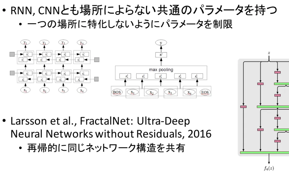
RNN, CNNとも場所によらない共通のパラメータを持つ

• 一つの場所に特化しないようにパラメータを制限

•

Larsson et al., FractalNet: Ultra-Deep

Neural Networks without Residuals, 2016

• 再帰的に同じネットワーク構造を共有

20 z f4pzq z f4pzq Block 1 Block 2 Block 3 Block 4 Block 5 x y

Fractal Expansion Rule

Layer Key Convolution Join Pool Prediction z fC fCpzq z fC fC fC`1pzq

Figure 1: Fractal architecture. Left: A simple expansion rule generates a fractal architecture with Cintertwined columns. The base case, f1pzq, has a single layer of the chosen type (e.g. convolutional)

between input and output. Join layers compute element-wise mean. Right: Deep convolutional networks periodically reduce spatial resolution via pooling. A fractal version uses fCas a building

block between pooling layers. Stacking B such blocks yields a network whose total depth, measured in terms of convolution layers, is B ¨ 2C´1_{. This example has depth 40 (B “ 5, C “ 4).}

The entirety of emergent behavior resulting from a fractal design may erode the need for recent engineering tricks intended to achieve similar effects. These tricks include residual functional forms with identity initialization, manual deep supervision, hand-crafted architectural modules, and student-teacher training regimes. Section2reviews this large body of related techniques. Hybrid designs could certainly integrate any of them with a fractal architecture; we leave open the question of the degree to which such hybrids are redundant or synergistic.

Our main contribution is twofold:

• We introduce FractalNet, the first alternative to ResNet in the realm of extremely deep convolutional neural networks. FractalNet is scientifically surprising; it shows that residual learning is not required for ultra-deep networks.

• Through analysis and experiments, we elucidate connections between FractalNet and an array of phenomena engineered into previous deep network designs.

As an additional contribution, we develop drop-path, a novel regularization protocol for ultra-deep fractal networks. Existing work on deep residual networks actually lacks demonstration of an effective regularization technique, instead relying solely on data augmentation [8,11]. In the absence of data augmentation, fractal networks, trained with dropout [10] and drop-path together, far exceed the reported performance of residual networks.

Drop-path constitutes not only an intuitive regularization strategy, but also provides means of optionally guaranteeing that trained fractal networks exhibit anytime behavior. Specifically, a particular schedule of dropped paths during learning prevents subnetworks of different depths from co-adapting. As a consequence, both shallow and deep subnetworks must individually produce correct output. Querying a shallow subnetwork at test time thus yields a quick and moderately accurate result in advance of completion of the full network.

ドロップアウト

[Srivastava et al., 2014]

• 訓練時にドロップアウト確率

(1-p)で隠れ変数hを0に置

換

• 事例毎に異なるネットワーク構造を評価・更新していることに

相当

• テスト時には学習結果パラメータを

p倍することで、擬似的に

複数のネットワークの幾何平均で予測していることに相当

à アンサンブル法

ドロップアウトなし ドロップアウト例1 ドロップアウト例₁ 21

最適化誤差に効く手法

初期値

• パラメータ行列は正規分布または一様分布からサンプ

リングすることが一般的

• パラメータのスケール（分散）が重要

• 小さすぎると誤差が伝わらない（Vanishing Gradient）

• 大きすぎると誤差が発散

(Exploding Gradient)

• 全ての層で活性化関数の分散と勾配の分散が等しく

なるようにするヒューリスティックス

•

Xavier initialization [Glorotand Bengio, 2010]

•

𝑊

_5f

~Uniform −

{ |

,

{ |

•

a=#input + #output

•

ReLU用初期値 [He et al., 2015]

•

𝑊

_5f

~𝑁 0,

p #5•€•‚ 23

Batch Normalization [Ioffe and

Szegedy, 2015]

• 隠れ変数を平均

0, 分散1に変換する層を追加

•

ℎ

ƒn1

＝

„…†‡ ˆ

• 平均

_{μ、分散σ}

2

_{はミニバッチ}

_{M個内で推定}

•

𝜇 =

_d1

∑ ℎ

ƒ(f) f

•

𝜎 = 𝜀 +

_d1

∑ ℎ

ƒ f

_{− 𝜇}

p f

•

εは 0を防ぐための微小な値

• すべての層の隠れ変数が同じ範囲だと微分も同じ範囲に

なりやすい

• 再掲

:

YG g H_YH

=

YG_YgYg_YH 24

例：活性化関数

𝜕𝑓

𝜕ℎ

= k

0,

ℎ ≤ 0

1,

ℎ > 0

例：行列・ベクトル積

𝜕𝑔

𝜕𝑥

= 𝑾

Batch Normalization and beyond

•

BNによって表現力が落ちないようにスケールとバ

イアスを加える

•

𝛼

„

…

†‡

ˆ

+ 𝛽

•

αとβはスカラーでW行列より学習が容易

• ミニバッチが不要な

BNの拡張：NormProp [Arpit et

al. 2016]

•

RNNなどは系列の長さが可変長だとミニバッチサイズも

ばらついてしまい

BNが使いづらい

• 入力を平均

_{0, 分散1の正規分布を仮定して、出力も平}

均

0, 分散1の正規分布になるように関数を解析的に変

更

25

Long Short-Term Memory (LSTM)

•

𝒊

_‚

𝒇

_‚

𝒐

_‚

𝒈

_‚

=

’5g“”5• 𝑾

’5g“”5• 𝑾

_•

I

𝒙

𝒙

—

_—

;𝒉

;𝒉

—š›

_—š›

n𝒃

n𝒃

I

_•

’5g“”5• 𝑾

_ž

𝒙

_—

;𝒉

_—š›

n𝒃

_ž

‚|•„ 𝑾

_Ÿ

𝒙

_—

;𝒉

_—š›

n𝒃

_Ÿ

•

𝒄

_‚

= 𝒇

_‚

∗ 𝒄

_‚†1

+ 𝒊

_‚

∗ 𝒈

_‚

•

𝒉

_‚

= 𝒐

_‚

∗ tanh 𝒄

_‚

•

LSTMではVanishing Gradientが起こりにくい理由

• 簡単のためf=1の場合:

𝒉

_‚

= 𝒉

_£

+ 𝒐

_‚

∗ tanh 𝒊

₁

∗ 𝒈

₁

+ 𝒊

_p

∗ 𝒈

_p

+ ⋯ + 𝒊

_‚

∗ 𝒈

_‚

•

Y𝒉

_—

YH

_›

=

Y𝒉

_¥

YH

₁

+

Y𝒐

_—

YH

₁

*

Y‚|•„

Y 𝒊

_›

∗𝒈

_›

n𝒊

_¦

∗𝒈

_¦

n⋯n𝒊

_—

∗𝒈

_—

Y𝒊

_›

∗𝒈

_›

YH

₁

+ ⋯

26

x

1

を変化させた時の時刻

tのh

t

への影響が直接的

時刻

_{1へのshort cutがある}

LSTM に関連した重要な手法

•

forget gate fのバイアスbは1に初期化する

•

Jozefowics et al. “An Empirical Exploration of Recurrent

Network Architectures”, 2015

•

𝒇

_‚

=

1

1n§H€ †𝑾

_•

𝒙

_—

;𝒉

_—š›

†𝒃

_•

•

b=1に初期化àfが1になりやすいà初期にvanishing gradient

が起きにくい

• メモリセル

cへのdropoutは更新分のみに適用する

•

Semeniuta et al., “Recurrent Dropout without Memory Loss”,

2016

•

𝒄

_‚

= 𝒇

_‚

∗ 𝒄

_‚†1

+ 𝑑𝑟𝑜𝑝𝑜𝑢𝑡(𝒊

_‚

∗ 𝒈

_‚

)

• 勧められないdropoutの適用

•

𝒄

_‚

= 𝑑𝑟𝑜𝑝𝑜𝑢𝑡(𝒇

_‚

∗ 𝒄

_‚†1

+ 𝒊

_‚

∗ 𝒈

_‚

)

•

𝒄

_‚

= 𝑑𝑟𝑜𝑝𝑜𝑢𝑡(𝒇

_‚

∗ 𝑑𝑟𝑜𝑝𝑜𝑢𝑡(𝒇

_‚†1

∗ 𝒄

_‚†p

+ 𝒊

_‚†1

∗ 𝒈

_‚†1

) + 𝒊

_‚

∗ 𝒈

_‚

)

• ・・・

•

t回dropoutを適用していることになり、0になる可能性が高い

27

ソフトアテンションモデル

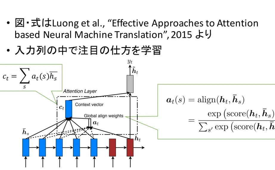
• 図・式は

_{Luong et al., “Effective Approaches to Attention}

based Neural Machine Translation”, 2015 より

• 入力列の中で注目の仕方を学習

28

with D being our parallel training corpus.

3 Attention-based Models

Our various attention-based models are classifed into two broad categories, global and local. These classes differ in terms of whether the “attention” is placed on all source positions or on only a few source positions. We illustrate these two model types in Figure 2 and 3 respectively.

Common to these two types of models is the fact that at each time step t in the decoding phase, both approaches first take as input the hidden state ht

at the top layer of a stacking LSTM. The goal is then to derive a context vector ct that captures

rel-evant source-side information to help predict the current target word yt. While these models differ

in how the context vector ct is derived, they share

the same subsequent steps.

Specifically, given the target hidden state ht and

the source-side context vector ct, we employ a

simple concatenation layer to combine the infor-mation from both vectors to produce an attentional hidden state as follows:

˜ht = tanh(Wc[ct; ht]) (5)

The attentional vector ˜ht is then fed through the

softmax layer to produce the predictive distribu-tion formulated as:

p(yt|y<t, x) = softmax(Ws˜ht) (6)

We now detail how each model type computes the source-side context vector ct.

3.1 Global Attention

The idea of a global attentional model is to con-sider all the hidden states of the encoder when de-riving the context vector ct. In this model type,

a variable-length alignment vector at, whose size

equals the number of time steps on the source side, is derived by comparing the current target hidden state ht with each source hidden state ¯hs:

at(s) = align(ht, ¯hs) (7)

= _Pexp score(ht, ¯hs)

s0 exp score(ht, ¯hs0)

Here, score is referred as a content-based function for which we consider three different alternatives:

score(ht, ¯hs) = 8 > < > : h>_t ¯hs dot h>_t Wa¯hs general Wa[ht; ¯hs] concat (8) yt ˜ht ct at ht ¯hs

Global align weights

Attention Layer

Context vector

Figure 2: Global attentional model – at each time step t, the model infers a variable-length align-ment weight vector at based on the current target

state ht and all source states ¯hs. A global context

vector ct is then computed as the weighted

aver-age, according to at, over all the source states.

Besides, in our early attempts to build attention-based models, we use a location-attention-based function in which the alignment scores are computed from solely the target hidden state ht as follows:

at = softmax(Waht) location (9)

Given the alignment vector as weights, the context vector ct is computed as the weighted average over

all the source hidden states.6

Comparison to (Bahdanau et al., 2015) – While our global attention approach is similar in spirit to the model proposed by Bahdanau et al. (2015), there are several key differences which reflect how we have both simplified and generalized from the original model. First, we simply use hidden states at the top LSTM layers in both the encoder and decoder as illustrated in Figure 2. Bahdanau et al. (2015), on the other hand, use the concatena-tion of the forward and backward source hidden states in the bi-directional encoder and target hid-den states in their non-stacking uni-directional de-coder. Second, our computation path is simpler; we go from ht ! at ! ct ! ˜ht then make

a prediction as detailed in Eq. (5), Eq. (6), and Figure 2. On the other hand, at any time t, Bah-danau et al. (2015) build from the previous hidden state ht 1 ! at ! ct ! ht, which, in turn,

6_{Eq. (9) implies that all alignment vectors a}

t are of the

same length. For short sentences, we only use the top part of a_t and for long sentences, we ignore words near the end.

1414

with D being our parallel training corpus.

3 Attention-based Models

Our various attention-based models are classifed

into two broad categories, global and local. These

classes differ in terms of whether the “attention”

is placed on all source positions or on only a few

source positions. We illustrate these two model

types in Figure 2 and 3 respectively.

Common to these two types of models is the fact

that at each time step t in the decoding phase, both

approaches first take as input the hidden state h

t

at the top layer of a stacking LSTM. The goal is

then to derive a context vector c

t

that captures

rel-evant source-side information to help predict the

current target word y

t

. While these models differ

in how the context vector c

t

is derived, they share

the same subsequent steps.

Specifically, given the target hidden state h

t

and

the source-side context vector c

t

, we employ a

simple concatenation layer to combine the

infor-mation from both vectors to produce an attentional

hidden state as follows:

˜h

_t

= tanh(W

c

[c

t

; h

t

])

(5)

The attentional vector ˜h

t

is then fed through the

softmax layer to produce the predictive

distribu-tion formulated as:

p(y

_t

_|y

_<t

, x) = softmax(W

s

˜h

t

)

(6)

We now detail how each model type computes

the source-side context vector c

t

.

3.1 Global Attention

The idea of a global attentional model is to

con-sider all the hidden states of the encoder when

de-riving the context vector c

t

. In this model type,

a variable-length alignment vector a

t

, whose size

equals the number of time steps on the source side,

is derived by comparing the current target hidden

state h

t

with each source hidden state ¯h

s

:

a

t

(s) = align(h

t

, ¯

h

s

)

(7)

=

_P

exp score(h

t

, ¯

h

s

)

s0

exp score(h

t

, ¯

h

s0

)

Here, score is referred as a content-based function

for which we consider three different alternatives:

score(h

_t

, ¯

h

s

) =

8

>

<

>

:

h

>_t

¯h

_s

dot

h

>_t

W

a

¯h

s

general

W

a

[h

t

; ¯h

s

] concat

(8)

y

t

˜h

_t

c

_t

a

t

h

t

¯h

_s

Global align weights

Attention Layer

Context vector

Figure 2:

Global attentional model – at each time

step t, the model infers a variable-length

align-ment weight vector a

t

based on the current target

state h

t

and all source states ¯h

s

. A global context

vector c

t

is then computed as the weighted

aver-age, according to a

t

, over all the source states.

Besides, in our early attempts to build

attention-based models, we use a location-attention-based function

in which the alignment scores are computed from

solely the target hidden state h

t

as follows:

a

_t

= softmax(W

a

h

t

)

location

(9)

Given the alignment vector as weights, the context

vector c

t

is computed as the weighted average over

all the source hidden states.

6

Comparison to (Bahdanau et al., 2015) – While

our global attention approach is similar in spirit

to the model proposed by Bahdanau et al. (2015),

there are several key differences which reflect how

we have both simplified and generalized from the

original model. First, we simply use hidden states

at the top LSTM layers in both the encoder and

decoder as illustrated in Figure 2. Bahdanau et

al. (2015), on the other hand, use the

concatena-tion of the forward and backward source hidden

states in the bi-directional encoder and target

hid-den states in their non-stacking uni-directional

de-coder. Second, our computation path is simpler;

we go from h

t

! a

t

! c

t

! ˜h

t

then make

a prediction as detailed in Eq. (5), Eq. (6), and

Figure 2. On the other hand, at any time t,

Bah-danau et al. (2015) build from the previous hidden

state h

t 1

! a

t

! c

t

! h

t

, which, in turn,

6

_{Eq. (9) implies that all alignment vectors a}

t

are of the

same length. For short sentences, we only use the top part of

a

_t

and for long sentences, we ignore words near the end.

1414

𝑐

_‚

= © 𝑎

_‚

(𝑠)ℎ

_’ ’

アテンションと

RNNによる生成の

組み合わせ

• 入力列から出力層への

shortcutを作っている とも考えら

れる

(Vanishing Gradientが起こりにくい）

29

A

RNN

Attention

A

RNN

Attention

encoder

_decoder

B

その他の

shortcut (skip

connection)を用いる手法

•

Residual Networks [He et al., 2016]

•

𝑓 𝑔 𝑥 + 𝑥

•

Highway Networks [Srivastava et al., 2015]

•

𝑓 𝑇(𝑥)𝑔 𝑥 + (1 − 𝑇(𝑥))𝑥

•

𝑇 𝑥 = sigmoid 𝑾𝑥 + 𝑏

• 重み付きのshortcut

• ただし、

shortcutはアンサンブル効果も

指摘されている

[Veit et al., 2016]

• 複数の深さの混ぜ合わせと見ることもできる

30

W

W

W

RNNの話題

•

RNNの可視化

•

RNN学習時に使われるヒューリスティックス

•

RNNはパラメータより状態保持にメモリが必要

• 言葉を生成する手法は出力層の計算・空間量が

重い

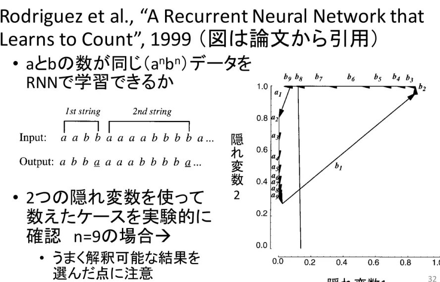
31

RNNは数を数えられるか

•

Rodriguez et al., “A Recurrent Neural Network that

Learns to Count”, 1999 （図は論文から引用）

•

_{aとbの数が同じ（a}

n

_b

n

_{）データを}

RNNで学習できるか

•

_{2つの隠れ変数を使って}

数えたケースを実験的に

確認

n=9の場合à

• うまく解釈可能な結果を

選んだ点に注意

₃₂

8

P. Rodriguez et al.

of performance, hence our analysis will show the nature of a solution that an RNN develops in this context.

In the rest of the paper, we describe the RNN simulation experiment, present some concepts from dynamical systems theory, and apply the concepts to the analysis of the RNN simulations. We focus the analysis on two network results for comparison and then, later, discuss two further experiments: one with another simple DCFL (a balanced parenthesis language) and one that explores learning issues with more hidden units. We also describe how the RNN dynamics represent a solution that can process extremely long strings under ideal conditions.

3. RNN Sim ulation Experiment

3.1. Issues

In this experiment we are concerned with the following two questions: (1) Can an RNN learn to process a simple DCFL with a prediction task? (2) What are the states and resources employed by the RNN?

The ®rst question demands that an RNN learn to process a simple DCFL so that it generalizes beyond those input/output mappings presented in training. In other words, the performance of the RNN must somehow re¯ect the underlying structure of the data. The second question demands a functional description of how the RNN re¯ects the structure of the data. Ideally, one should ground the functional description of states and resources on a formal analysis of the RNN dynamics. First, we describe an RNN experiment to address the ®rst question; later, we describe some standard features of dynamical systems theory as the method of analysis to address the second question.

3.2. Simulation Details

3.2.1. The input±output mapping task. The input stimuli consisted of strings from a very simple DCFL that uses two symbols, {a,b}, of the form an

bn. The input is presented one character at a time and the output of the network is trained to predict the next input in the sequence. Since the network outputs are not strictly binary, a correct prediction has a threshold value of 0.5. An example of the input±output mappings for network training is the following:

(note the transition at the last b should predict the ®rst a of the next string).

Notice that when the network receives an a input, it will not be able to predict accurately the next symbol because the next symbol can be either another a or the ®rst b in the sequence. On the other hand, when the network receives a b input it should accurately predict the number of b symbols that match the number of a inputs already seen, and then also predict the end of the string (Batali, 1994). Correct processing to accept a string is de®ned as follows:

16 P. Rodr iguez et al.

chosen by allowing the network to run for one or two short strings. Importantly, for each string the last b input causes a change in {HU1,HU2} that crosses over to the left of the dividing line, hence the network properly predicts an a when the last b is input. Not surprisingly, the last {HU1,HU2} value is near the initial starting value.

Figure 5 shows the trajectories for n5 8 and n5 9. Note that the trajectory steps are increasingly shorter near the Fa attracting ®xed point. Also, the ®rst b

input causes a transition to a region of phase space where the trajectory can take

Figure 5. Network 1 trajectories for n5 8 and n5 9. For n5 8, the trajectory crosses the dividing line on only the last arrow; but for n5 9 the trajectory crosses the line on the eighth b input, which is one time step too early. For n > 9 the network had similar results of making predictions for the start of the next string too early.

隠れ変数

₁

隠

れ

変

数

2

RNN文字言語モデルの可視化

•

Karpathy et al., “Visualizing and Understanding Recurrent Networks”,

2016. (図は論文より引用)

•

LSTMのセルの値を可視化（うまく解釈可能な結果を選んだ

点に注意）

• 文末・引用符に反応するセル

33

Figure 2: Several examples of cells with interpretable activations discovered in our best Linux

Ker-nel and War and Peace LSTMs. Text color corresponds to tanh(c), where -1 is red and +1 is blue.

Figure 3:

Left three: Saturation plots for an LSTM. Each circle is a gate in the LSTM and its

position is determined by the fraction of time it is left and right-saturated. These fractions must add

to at most one (indicated by the diagonal line).

Right two: Saturation plot for a 3-layer GRU model.

1. n-NN: A fully-connected neural network with one hidden layer and tanh nonlinearities. The

input to the network is a sparse binary vector of dimension nK that concatenates the one-of-K

encodings of n consecutive characters. We optimize the model as described in Section 3.3 and

cross-validate the size of the hidden layer.

2. n-gram: An unpruned (n + 1)-gram character-level language model using modified

Kneser-Ney smoothing (3). This is a standard smoothing method for language models (15). All models

were trained using the popular KenLM software package (13).

Performance comparisons. The performance of both n-gram models is shown in Table 2. The

n-gram and n-NN models perform nearly identically for small values of n, but for larger values

the n-NN models start to overfit and the n-gram model performs better. Moreover, we see that on

both datasets our best recurrent network outperforms the 20-gram model (1.077 vs. 1.195 on WP

and 0.84 vs.0.889). It is difficult to make a direct model size comparison, but the 20-gram model

file has 3GB, while our largest checkpoints are 11MB. However, the assumptions encoded in the

Kneser-Ney smoothing model are intended for word-level modeling of natural language and may

not be optimal for character-level data. Despite this concern, these results provide some evidence

that the recurrent networks are effectively utilizing information beyond 20 characters.

Error Analysis. It is instructive to delve deeper into the errors made by both recurrent networks and

n-gram models. In particular, we define a character to be an error if the probability assigned to it

by a model is below 0.5. Figure 4 (left) shows the overlap between the test-set errors for the 3-layer

LSTM, and the best n-NN and n-gram models. We see that the majority of errors are shared by all

three models, but each model also has its own unique errors.

5

Figure 2: Several examples of cells with interpretable activations discovered in our best Linux

Ker-nel and War and Peace LSTMs. Text color corresponds to tanh(c), where -1 is red and +1 is blue.

Figure 3:

_{Left three: Saturation plots for an LSTM. Each circle is a gate in the LSTM and its}

position is determined by the fraction of time it is left and right-saturated. These fractions must add

to at most one (indicated by the diagonal line).

_{Right two: Saturation plot for a 3-layer GRU model.}

1. n-NN: A fully-connected neural network with one hidden layer and tanh nonlinearities. The

input to the network is a sparse binary vector of dimension nK that concatenates the one-of-K

encodings of n consecutive characters. We optimize the model as described in Section 3.3 and

cross-validate the size of the hidden layer.

2. n-gram: An unpruned (n + 1)-gram character-level language model using modified

Kneser-Ney smoothing (3). This is a standard smoothing method for language models (15). All models

were trained using the popular KenLM software package (13).

Performance comparisons. The performance of both n-gram models is shown in Table 2. The

n-gram and n-NN models perform nearly identically for small values of n, but for larger values

the n-NN models start to overfit and the n-gram model performs better. Moreover, we see that on

both datasets our best recurrent network outperforms the 20-gram model (1.077 vs. 1.195 on WP

and 0.84 vs.0.889). It is difficult to make a direct model size comparison, but the 20-gram model

file has 3GB, while our largest checkpoints are 11MB. However, the assumptions encoded in the

Kneser-Ney smoothing model are intended for word-level modeling of natural language and may

not be optimal for character-level data. Despite this concern, these results provide some evidence

that the recurrent networks are effectively utilizing information beyond 20 characters.

Error Analysis. It is instructive to delve deeper into the errors made by both recurrent networks and

n

-gram models. In particular, we define a character to be an error if the probability assigned to it

by a model is below 0.5. Figure 4 (left) shows the overlap between the test-set errors for the 3-layer

LSTM, and the best n-NN and n-gram models. We see that the majority of errors are shared by all

three models, but each model also has its own unique errors.

RNNの学習時によく使われる

ヒューリスティックス

•

Truncated Backpropagation Through Time (BPTT)

(Elman (1990) , Mikolov et al., 2010)

• 誤差逆伝播をFステップ毎にB時刻分行う

•

for t in 1…T

•

forwardprop: ℎ

𝑡

= 𝑅𝑁𝑁 ℎ

‚†1

, 𝑥𝑡

•

if t % F == 0 then

•

for s in t ... t – B; backprop

•

end

•

exploding/ vanishinggradient に有効

•

gradient norm clipping (Pascanu et al., 2013)

• 勾配ベクトルgのノルムに閾値を設けて、超えたらスケール

する

•

if 𝒈 ≥ threshold then

• 𝒈 = threshold 𝐠 𝒈

•

explodinggradient に有効

34

RNN実装の課題: メモリ使用量

• 入力・隠れ変数の数

H=256, 出力サイズ|Y|=10K

• ミニバッチサイズ

B=32, 長さT=64

•

RNN: y

_t

= o(𝐖

_o

f 𝐖

_r

𝒙

_‚

; 𝒉

_‚†1

)

• パラメータ数

:

•

_|W

_r

_{|= H * 2H = 128K}

•

_|W

_o

_{|=H * |Y| = 2500K}

•

Backprop用状態変数

•

_{H * B * T = 512K}

•

|Y| * B * T = 20000K

35

RNNはパラメータよりBackprop用の状態保持にメモリが必要

単語を出力するモデルの場合

出力層のメモリ使用量が問題となる

• 出力サイズ

|Y|=800K (頻度3以上の単語のみ)

•

1 billion word language modeling benchmark [Chelba et

al., 2013]

https://github.com/ciprian-chelba/1-billion-word-language-modeling-benchmark

• 出力層パラメータ数

_{: |W}

_o

_{|=H * |Y| = 194M}

• 出力層状態変数

|Y| * B * T = 1.464G

• 最新

GPUでもメモリ搭載量は12-16GB程度

• 出力層の状態変数 を抑える手法が必要

36

出力層の状態変数 を抑える手

法

• 階層ソフトマックス （

Hierarchical Softmax）

Goodman 2001, Mikolov et al. 2011

•

_{yをクラスタリングし、クラスタc(y)を定義}

• 階層化

_{: p(y|x) = p(c(y)|x) p(y|c(y))}

• クラスタ数を

|𝑌|とすれば2 |𝑌| ≪ |Y|に抑えられる

• クラスタは頻度などで決定

• サンプリング法

Jozefowicz et al. 2016, Ji et al. 2016

•

ℓ

_𝜃

𝑥

(5)

, 𝑦

(5)

= −log

DEF G

?

H

(I)

,J

(I)

DEF G

_?

H

(I)

_,J

(I)

_n∑

_{DEF G}

?

H

(I)

,JK

LM∈¶

•

𝑆 ∈ 𝑌 ∖ 𝑦

(5)

: 全出力を使わずに部分集合を使用

• 部分集合は頻度に基づきサンプリングすることが多い

• 学習時のメモリ・計算量を減らす手法

37

文字単位で予測する手法

• 単語単位

: |Y| = 単語異なり数 1万以上

• 未知語の問題（通常は低頻度語を未知語として学習）

• 語形変化を扱えない（

_{wordとwordsは別々のシンボル）}

• 文字単位

: |Y| = 文字異なり数

• 訓練データにでてこない文字は稀、語形変化を学習で

きる可能性

•

Chung et al. “A Character-Level Decoder without

Explicit Segmentation for Neural Machine

Translation”, 2016.

•

En-Cs, En-De, En-Fi で最先端の性能を達成

38

まとめ

•

RNNの可視化

•

RNN学習時に使われるヒューリスティックス

•

RNNはパラメータより状態保持にメモリが必要

• 言葉を生成する手法は出力層の計算・空間量が

重い

39

オススメの教科書

•

Ian Goodfellow, Yoshua Bengio, and Aaron Courville.

Deep Learning. MIT Press, 2016.

•

online version (free):

http://www.deeplearningbook.org/

40

参考文献

•

Ilya Sutskever, Oriol Vinyals, and Quoc V. V Le.

“Sequence to sequence learning with neural

networks”. NIPS 2014.

•

Gustav Larsson, Michael Maire, and Gregory

Shakhnarovich. “FractalNet: Ultra-Deep Neural

Networks without Residuals”. arXiv:1605.07648,

2016.

•

Nitish Srivastava, Geoffrey Hinton, Alex Krizhevsky,

Ilya Sutskever, Ruslan Salakhutdinov. “Dropout: A

Simple Way to Prevent Neural Networks from

Overfitting”. JMLR, 15(1), 2014.

41

参考文献

• Xavier Glorot and Yoshua Bengio. “Understanding the difficulty of training deep feedforward neural networks”, In Proc. of AISTATS 2010.

• Kaiming He, Xiangyu Zhang, Shaoqing Ren, and Jian Sun. “Delving Deep into Rectifiers:

Surpassing Human-Level Performance on ImageNet Classification”, arXiv:1502.01852, 2015. • Sergey Ioffeand Christian Szegedy. “Batch Normalization: Accelerating Deep Network Training by

Reducing Internal Covariate Shift”. In Proc. of ICML 2015.

• Devansh Arpit, Yingbo Zhou, Bhargava U. Kota, Venu Govindaraju. “Normalization Propagation: A Parametric Technique for Removing Internal Covariate Shift in Deep Networks”. In Proc. of ICML 2016.

• Rafal Jozefowicz, Wojciceh Zaremba, and Ilya Sutskever. “An Empirical Exploration of Recurrent Network Architectures”, In Proc. of ICML 2015.

• Stanislau Semeniuta, Aliaksei Severyn, Erhardt Barth. “Recurrent Dropout without Memory Loss”. arXiv:1603.05118, 2016.

• Minh-Thang Luong, Hieu Pham, and Christopher D. Manning. “Effective Approaches to Attention-based Neural Machine Translation”, In Proc. of EMNLP 2015.

• Kaiming He, Xiangyu Zhang, Shaoqing Ren, and Jian Sun. “Identity Mappings in Deep Residual Networks”. arXiv:1603.05027, 2016.

• Rupesh Kumar Srivastava, Klaus Greff, and Jürgen Schmidhuber. “Training Very Deep Networks”. NIPS 2015.

• Andreas Veit, Michael Wilber, Serge Belongie, “Residual Networks are Exponential Ensembles of Relatively Shallow Networks”, arXiv:1605.06431, 2016.

参考文献

• Paul Rodriguez , Janet Wiles, and Jeffrey L. Elman. “A Recurrent Neural Network that Learns to Count”. Connection Science 11 (1), 1999.

• Andrej Karpathy, Justin Johnson, and Li Fei-Fei. “Visualizing and Understanding Recurrent Networks”. In Proc. of ICLR2016 Workshop.

• Jeffrey L. Elman. “Finding structure in time”. Cognitive science, 14(2), 1990.

• Tomas Mikolov, Martin Karafiat, Kukas Burget, Jan “Honza” Cernocky, Sanjeev Khudanpur : Recurrent Neural Network based Language” In Proc. of INTERSPEECH 2010.

• Razvan Pascanu, Tomas Mikolov, and Yoshua Bengio. “On the difficulty of training Recurrent Neural Networks”, In Proc. of ICML 2013.

• Ciprian Chelba, Tomas Mikolov, Mike Schuster, Qi Ge, Thorsten Brants, Phillipp Koehn, and Tony Robinson. “One Billion Word Benchmark for Measuring Progress in Statistical Language Modeling”, arXiv:1312.3005, 2013. • Joshua Goodman. “Classes for Fast Maximum Entropy Training”. In Proc. of ICASSP 2001.

• Tomas Mikolov, Stefan Kombrink, Lukas Burget, Jan Cernocky, and Sanjeev Khudanpur. “Extensions of Recurrent Neural Network Language Model”. In Proc. of ICASSP 2011.

• Rafal Jozefowicz, Oriol Vinyals, Mike Schuster, Noam Shazeer, and Yonghui Wu. “Exploring the Limits of Language Modeling”. arXiv: 1602.02410. 2016.

• Shihao Ji, S. V. N. Vishwanathan, Nadathur Satish, Michael J. Anderson, and Pradeep Dubey. “BlackOut:

Speeding up Recurrent Neural Network Language Models With Very Large Vocabularies”. In Proc. of ICLR 2016. • Junyoung Chung, Kyunghyun Cho, and Yoshua Bengio. “A Character-Level Decoder without Explicit

Segmentation for Neural Machine Translation”, 2016.