Complex temporal patterns in molecular dynamics: A direct measure of the phase-space
exploration by the trajectory at macroscopic time scales
Dmitry Nerukh
*
Unilever Centre for Molecular Informatics, Department of Chemistry, Cambridge University, Cambridge CB2 1EW, United Kingdom
Vladimir Ryabov
School of Systems Information Science, Department of Complex Systems, 116-2 Kamedanakano-cho, Hakodate-shi, 041-8655 Hakodate, Hokkaido, Japan
Robert C. Glen
Unilever Centre for Molecular Informatics, Department of Chemistry, Cambridge University, Cambridge CB2 1EW, United Kingdom 共Received 18 July 2007; revised manuscript received 13 November 2007; published 28 March 2008兲
Computer simulated trajectories of bulk water molecules form complex spatiotemporal structures at the picosecond time scale. This intrinsic complexity, which underlies the formation of molecular structures at longer time scales, has been quantified using a measure of statistical complexity. The method estimates the information contained in the molecular trajectory by detecting and quantifying temporal patterns present in the simulated data 共velocity time series兲. Two types of temporal patterns are found. The first, defined by the short-time correlations corresponding to the velocity autocorrelation decay times共ⱕ0.1 ps兲, remains asymp-totically stable for time intervals longer than several tens of nanoseconds. The second is caused by previously unknown longer-time correlations 共found at longer than the nanoseconds time scales兲 leading to a value of statistical complexity that slowly increases with time. A direct measure based on the notion of statistical complexity that describes how the trajectory explores the phase space and independent from the particular molecular signal used as the observed time series is introduced.
DOI:10.1103/PhysRevE.77.036225 PACS number共s兲: 05.45.Jn, 83.10.Rs, 61.20.Ja, 02.70.Ns
I. INTRODUCTION
Molecular dynamics共MD兲 trajectories representing a dif-fusion process in liquids form complex patterns in the phase space. Because of the system’s high dimensionality共defined by the number of interacting molecules in the analyzed vol-ume兲, single molecule trajectories in the long-time limit are usually assumed to be indistinguishable from correlated noise by standard statistical methods关1兴. However, the equa-tions of motion of each particle are deterministic, therefore, the local nonlinear dynamics at the picosecond time scale may lead to nontrivial behavior and the emergence of mo-lecular structures over much longer共nanoseconds兲 periods. Discovering and quantifying this nontrivial long-term behav-ior and intrinsic complexity of molecular trajectories 共over various time scales兲 that can shed light on the origin of emer-gent molecular behavior is the subject of the present work.
The computational mechanics approach suggested by Crutchfield et al. 关2–4兴 seems to be most suitable for the task. The approach is useful for detecting dynamical struc-tures in observed time series, since it is based on information-theoretic concepts, without detailed assumptions on the geometric properties of the structures originating from the dynamics in the phase space. The authors introduced the idea of an⑀machine working in the space of so-called causal states that catch the principal dynamics of the system. One of the central concepts of the formalism is a statistical complex-ity measure, a characteristic of the⑀machine, that describes
how complex the underlying process is by quantifying the amount of information stored and processed by the system. The advantage of computational mechanics is that, besides intuitive共and at the same time mathematically rigorous兲 sta-tistical properties that quantify the complexity, it captures complete statistical information contained in the signal共see the Appendix兲.
It should be noted that there exist several alternative defi-nitions of complexity used in different contexts. The analysis of the metric properties of sets of trajectories in phase space 关5兴 or the study of time separation between initially close trajectories 关6兴 should be distinguished from the statistical complexity used in the present work. The latter is aimed at purely probabilistic modeling of the time series, irrespective of the geometry of trajectories in the phase space or local instability of the dynamics. Approaches for estimating the physical complexity of classical trajectories using their information-theoretic contents include, for example, work by Brudno关7兴 that relates Kolmogorov’s algorithmic complex-ity and the metric entropy of an ergodic dynamical system. Recently, Segre关8兴 showed that chaotic dynamical systems are simple from Bennett’s “logical depth” point of view. Benci et al.关9兴 have investigated the amount of information necessary to describe the chaotic orbits and find more than logarithmic increase with time for weakly chaotic cases.
An alternative approach to the analysis of molecular tra-jectories could be the application of the concepts and meth-ods of time series analysis that appeared recently in the field of nonlinear dynamics for characterizing intrinsically deter-ministic processes关10,11兴. However, this group of time se-ries analysis techniques seems to be feasible only for systems *dn232@cam.ac.uk
with few degrees of freedom. The limitation of all nonlinear dynamics methods is the assumption of the existence of a low-dimensional manifold 共attractor兲 in the phase space where the essential dynamics occur. It is, however, unclear whether this concept can be effectively utilized in a numeri-cal analysis of signals obtained from highly dimensional sys-tems, such as fully developed turbulence, the human brain, or molecular ensembles. It is, therefore, necessary to search for new techniques that would discover inherent signatures of dynamics rather than assume the existence of structures in the phase space.
From the viewpoint of classical physics, the motion of a single particle 共hydrogen atom in our case兲 in bulk water without impurities can be well approximated by a stochastic model of Brownian motion. Characterizing a molecular tra-jectory in terms of diffusion theory reveals linear time growth of the mean square displacement关12兴, that approxi-mately corresponds to theoretical predictions from the clas-sical theory of Brownian motion 关13兴. Although deviations from Gaussianity of corresponding distribution functions can be detected by the analysis of higher moments 关1,14兴 the experimental共or numerically simulated兲 time series becomes indistinguishable from a stochastic Gaussian process at time periods longer than⬇100 ps 共at room temperature兲 关1,15兴. This implies a sufficient description of molecular trajectories in terms of correlation functions and/or power spectra and almost trivial behavior on the time scales larger than “corre-lation time” defined by, e.g., the first zero of the autocorre-lation function.
Although such a stochastic approach provides a satisfac-tory description of liquids at the macroscopic scale, there is no clear understanding of how the observed macroscopic randomness is produced by purely deterministic equations of motion of every atom, i.e., how the microscopically ordered motion is transformed to the macroscopic disorder. There were several attempts recently to demonstrate that at a mi-croscopic level the motion of molecules is chaotic关16兴, and the randomness due to local instability of trajectories in the phase space is transformed to a random walk motion of Brownian particles observed in experiments. It has been ar-gued, however, in later works 关17兴 that similar random be-havior at macro level can be caused by nonchaotic systems that do not possess the property of local instability at micros-cales. Therefore, the question on the microscopic origin of macroscopic randomness remains open.
On the other hand, it became clear recently关18兴 that, even if the dynamics of a single microparticle is chaotic its tem-poral behavior may be nontrivial due to the presence of reso-nances in the phase space and particles can demonstrate anomalous diffusion. When a chaotically moving particle comes close to any of the resonance zones, it can spend an abnormally long time there due to the so-called “stickiness” of the border of the resonances. As a result of such intermit-tent behavior, the phase space becomes strongly nonuniform and processes with significantly different characteristic tem-poral scales appear in the time series representing the trajec-tories. Consequently, particle trajectories may possess much longer memories than can be expected from a simple analy-sis of the autocorrelation function.
All the above considerations provide motivation for per-forming the analysis of molecular trajectories over very
long-time periods compared to time scales defined by the autocorrelation functions 共⬇1 ps兲, aimed at detecting non-trivial共i.e., different from a pure Gaussian noise兲 temporal structures. In order to quantify the deterministic origin of the dynamics of particles in a high-dimensional phase space cor-responding to MD trajectories of bulk water we apply a com-bination of the computational mechanics approach and a sur-rogate data method from nonlinear dynamics关19兴. Our goal is to detect and quantify complex temporal structures present in the water trajectory defined by the deterministic dynamics. We show that, because of existing long-time correlations, the structure of the groups of histories, the⑀machine, in the MD signal is qualitatively different from that obtained for an ar-tificial random time series共surrogate兲 with identical correla-tion and/or spectral properties.
Our work can thus serve to provide insights into two im-portant open problems:共i兲 is it possible to apply the compu-tational mechanics approach to realistic molecular systems; 共ii兲 does computational mechanics give a possibility to quan-tify nontrivial temporal structures in liquid water.
The next section describes the specifics about the molecu-lar model for water used in our calculations, as well as other details of numerical procedures used to obtain the molecular trajectory. The main idea and the methodology of the further analysis aimed at quantifying the informatic-theoretical con-tent of the calculated time series are given in Sec. III. The obtained results are presented in Secs. IV and V, while their interpretation is provided in Sec. VI.
II. MOLECULAR MODEL AND MOLECULAR DYNAMICS SIMULATION DETAILS
Water, being a complex liquid, has arguably one of the most developed simulation models关20–27兴. Numerous MD models of water differ in sophistication depending on the specific task of the simulation. For us, the combination of the simulation speed and the potential ability of modeling pro-tein folding was decisive in choosing the molecular model. We, therefore, focused on simple point charge 共SPC兲 关28兴 water while checking other flavors for the consistency of the results. We expect that the main conclusions of this work will hold for other liquids, the extensive study of which is, how-ever, a subject of a separate publication.
Bulk water consisting of 392 or 878 SPC, simple point charge extended共SPC-E兲 关28兴, or transferable intermolecular potential 3 point共TIP3P兲 molecules was simulated using the GROMACS molecular dynamics 关29兴 package. The tempera-ture of the system was kept constant at 275, 300, or 380 K using Berendsen关30兴 or Nose-Hoover 关31兴 thermostats, with a coupling time of 0.1 ps, whose combination with various coupling constants was investigated. Pressure coupling was also applied to a pressure bath with a reference pressure of 1 bar and a coupling time of 0.1 ps. A 1 nm cutoff distance for both van der Waals and Coulomb potentials was used. An equilibration until the potential and kinetic energies reach constant levels of fluctuations was performed before collect-ing data for analysis. The velocity of the oxygen and hydro-gen atoms of one of the water molecules was used as a three-dimensional signal for the complexity analysis. Instant
temperature, Tinst= 1 Ndfk兺imivi
2, where the summation is over all atoms, Ndf is the number of degrees of freedom and k is the Boltzman constant, was also used for calculating the complexity values.
Classical molecular systems are Hamiltonian. However, numerical errors associated with the model potential and thermostatting algorithm make the simulated MD system non-Hamiltonian. Therefore, we use a selected velocity sub-space for building a symbolic sequence and reconstructing the phase space without recourse to the Hamiltonian proper-ties of the underlying molecular dynamics.
III. IDEA AND METHODOLOGY A. Signal analysis
1. Diffusion process
Traditionally, motion of a single particle in a liquid that appears random can be characterized by the time dependence of its mean squared displacement具x2共t兲典, which demonstrates a power law behavior
具x2共t兲典 ⬀ t␣ 共1兲
at sufficiently long times. Here x共t兲 corresponds to the devia-tion of the coordinate x from the arbitrary initial condidevia-tion
x共0兲 and the averaging is performed either over an ensemble
of trajectories, or, under the assumption of ergodicity of the diffusion process, over an ensemble of initial conditions along a single trajectory. Normal diffusion 共Brownian mo-tion兲 then corresponds to the value of the diffusion coeffi-cient␣= 1, whereas values different from unity indicate the presence of anomalous diffusion. The case of 0⬍␣⬍1 is called subdiffusion, whereas the range of values 1⬍␣⬍2 is attributed to a superdiffusion process. The limiting value of
␣= 2 characterizes the ballistic regime typical to free motion of the particles over short distances. Note that the distribu-tion of x共t兲 is Gaussian only in the asymptotic limit of t
→⬁ and at small t significant deviations from Gaussianity
can be detected by the analysis of higher moments关1兴. The indicator共t兲 is often used for quantifying the non-Gaussian behavior关12,14兴
共t兲 = 具x4共t兲典
3具x2共t兲典− 1. 共2兲
Due to the fact that for a Gaussian distribution 具x4共t兲典 = 3具x2共t兲典, the deviation of the indicator 共t兲 from zero is a manifestation of intrinsic non-Gaussianity of the process
x共t兲.
2. Phase-space partitioning
In this study the velocity of one of the atoms is mainly used as a three-dimensional signal for the complexity analy-sis. The domain of the signal values appearing in the simu-lation has the shape of a ball centered at the origin with the radius of⬇4 nm/ps. The approximately centrally symmetric distribution of the data points makes the velocities a conve-nient signal for symbolization and data accumulation in
con-trast to, for example, the coordinates that diffuse very slowly in the phase space.
At the initial stage of data analysis, the original three-dimensional vector time series is transformed to a scalar symbolic sequence. The symbols are produced by applying a special phase-space coarse graining procedure on a suitably chosen cross section plane in the velocity space. It turns out that if thevz= 0 plane is used as a section surface, the aver-age time interval between the resulting data points 共⬇0.032 ps兲 roughly corresponds to the first minimum on the autocorrelation function of the original three-dimensional signal. A natural choice for the phase-space partitioning used for symbolization would be the generating partition 共GP兲 关32兴 that has the property of a one-to-one correspondence between the continuous trajectory and the generated sym-bolic sequence. That is, all information is retained after the symbolization. However, because of the very high dimen-sionality of the system it is infeasible to find a GP in our case. There are methods for calculating approximations to the GP. Using one of them关33兴 we obtained indications of what an optimal partition would look like. For our velocities data, the resulting approximated GPs were centrally symmet-ric for all tested number of partitions; the cases for two, three, four, and five partitions are shown in Fig.1. Thus, for all the data analyzed we used centrally symmetrical parti-tions for converting the continuous data into symbolic se-quences.
Summarizing, the following procedure was used for sym-bolization共Fig.1兲: 共i兲 the velocities of the hydrogen 共or oxy-gen兲 atoms were used as a continuous three-dimensional sig-nal; 共ii兲 at the locations where the velocity pierces the xy plane the points of the map were generated; 共iii兲 using the centrally symmetric partitions the map was converted into the symbolic sequence. The size K of the alphabet to be used in the conversion process is empirically found to be suffi-cient at the value K = 3 for good convergence and reproduc-ibility of numerical results.
3. Reconstruction of the⑀ machine
Computational mechanics detects hidden order within random looking symbolic sequences by building a linked
vx
vz
vy
v
FIG. 1. 共Color兲 Approximations for generating partitions ob-tained using the method by Buhl and Kennel 关33兴 for the cross
section of the hydrogen velocity space for the partitions correspond-ing to two-, three-, four-, and five-symbols alphabet.
structure of probabilistically related states in the phase space, the⑀ machine. The phase space is obtained by a procedure similar to the attractor reconstruction technique in dynamical systems theory based on the Takens embedding theorem 关34兴, but with a symbolic sequence taken for an original time series. Every point in an l-dimensional reconstructed phase space then corresponds to a set of l successive symbols from the共scalar兲 symbolic sequence.
Such sets of symbols共heretofore, histories of length l兲 are grouped according to their ability to predict one step for-ward. If the time step between successive symbols approxi-mately equals the correlation decay time, then, e.g., for a completely random process, all the histories are grouped into a single causal state. Due to the absence of predictive power on the time scales longer than the decay time of correlations, this simply reflects the fact that all histories predict the same random futures.
Contrary to completely random signals, the groups of his-tories with similar futures are numerous for the molecular signal, and corresponding causal states can be characterized by their occurrence rates P共⑀i兲 共see the Appendix兲. The sta-tistical complexity Cis then a statistical measure quantify-ing the difference of the distribution of P共⑀i兲 from the uni-form one expected for a purely stochastic process. Therefore, as will be shown in subsequent sections, the difference of the molecular signal from a random signal consists of both the large number of unique causal states found in the phase space, and the corresponding high value of the statistical complexity.
4. Surrogate time series analysis
It should be noted that the algorithms used for numerical identification of the set of causal states and estimating the value of statistical complexity include several computational steps as well as many internal parameters that control the computation precision and statistical confidence of the re-sults. As a consequence, there are a number of potential sources for statistical errors and biases that require special care. A straightforward approach would be direct analysis of corresponding distribution functions for the estimated values, with the subsequent calculation of moments共including dis-persion兲 and the associated error bars. However, this type of analysis encounters serious technical difficulties due to the complexity of the calculation procedure that is, in fact, a combination of several algorithms. We therefore accepted a different, much simpler way of getting error estimates, widely used in the literature on the analysis of time series. In works devoted to statistical data analysis, it is also known as the “bootstrap” method 关35兴, whereas in papers discussing nonlinear dynamics based techniques 关19兴 it is called the “surrogate data” method. Throughout this paper, we use the latter term as the name for artificial time series.
The idea of the surrogate data methodology consists of the comparison of the experimental data to a set of artifi-cially created time series 共surrogates兲, which lack some in-trinsic property of interest but have very similar 共or even identical兲 probability density function and/or power spec-trum to those of the original data. This method thus provides a kind of “control experiment” that allows testing of the
experimental time series against a hypothesis that it is pro-duced by a linear stochastic process like, e.g., an autoregres-sive moving average process共ARMA兲 关36兴.
The practical algorithm implementing the idea of surro-gate data consists of several steps. First, a statistical indicator called discriminating statistics has to be defined. From a gen-eral viewpoint of time series analysis, this could be any real number calculated from the data, like, for example, a high-order moment, autocorrelation, fractal dimension, or statisti-cal complexity, depending on the particular property of inter-est that the analysis is focused on. At the second stage, the surrogate data series are produced by using a random number generator combined with some original algorithm of data transformation. In other words, the algorithm converts the random sequence of numbers to a time series with required properties. The surrogates preserve some well-controlled sta-tistical characteristics of the analyzed data, but lack the prop-erty of interest. For example, in the context of the analysis of deterministic dynamics, the surrogates are usually chosen to have the power spectrum identical to the original data series, but, by its definition, do not possess any property imposed by deterministic dynamics such as, e.g., finite value of correla-tion dimension 关37兴 or others 关38兴. At the final stage, the discriminating statistics have to be calculated for original data and compared to a set of corresponding values calcu-lated from a set of surrogate time series. Significant discrep-ancy in the calculated values can be considered as an indi-cation of an essential difference between the surrogates and the original time series in the analyzed property.
In this work the discriminating statistics are the number of causal states nst and the value of statistical complexity C. For surrogates, we use two types of time series:
共1兲 Phase-shuffled surrogate. This is a standard surrogate time series obtained via the phase-shuffling algorithm关19兴. The data obtained with this method possess identical power spectrum共and, hence, autocorrelation function兲 to the origi-nal time series, but lack the property of dynamic correlation between the data points. It is generated by calculating the Fourier spectrum of the original data and assigning random values to all the phases of Fourier components. After calcu-lating the inverse Fourier transform, the artificial data series 共surrogate兲 has the unchanged power spectrum but is com-pletely random, i.e., it belongs to the class of Gaussian linear stochastic processes.
共2兲 Temporal pattern-shuffled surrogate. This surrogate data set is created by introducing random perturbations to the original time series that do not change dynamic temporal patterns in the data up to a certain time period Tr. It is ob-tained by random rotation共by a random angle兲 of the data segments containing nrconsecutive points in the phase-space cross-section plane共see Fig.1兲. The surrogates obtained by this method allow an analysis of the relationship between the characteristic periods in the analyzed data and the structure of causal states in the⑀machine.
IV. RESULTS
A. Overview of the dynamics and statistical analysis
1. Spectral characteristics
The velocity autocorrelation functions共vacf兲 of water at-oms, obtained as a time average over 2 ns共Fig.2兲, show that
linear time correlations last for⬇0.2 ps for the hydrogens and ⬇0.5 ps for the oxygens. From a viewpoint of linear correlation theory, there are no long-range temporal correla-tions in the analyzed data.
On the other hand, the power spectrum of the velocity fluctuations共Fig.3兲 shows a nontrivial feature at somewhat longer time scales: a broad low frequency peak is present at ⬇1 ps.
This fact can also be visualized by plotting the trajectory corresponding to the time evolution of the orientation vector of a water molecule共Fig.4兲. The trajectory shown in Fig.4 clearly displays complicated intermittent dynamical struc-tures over different time scales. A typical temporal pattern observed for such data can be roughly described as follows. It tends to fluctuate around some fixed value for a time pe-riod of⬇1 ps demonstrating quick jumps to other areas of similar fluctuations within a much shorter time interval 共compared to 1 ps兲. Note, that such behavior can be a mani-festation of a fractional kinetics process typical to Hamil-tonian systems typically containing resonances关39兴.
2. Diffusion
The calculation of the squared displacement for a hydro-gen atom shows a power law behavior, implying a diffusion process with the diffusion constant slightly less than unity, Fig.5. The largest deviation from the normal diffusion with
␣= 1 is observed at the time scales approximately corre-sponding to the maximum in the power spectrum, i.e., at about 1 ps. Therefore, the Brownian motion of the hydrogen atom can be roughly classified as normal diffusion at time scales longer than ⬇100 ps. At long time scales 共ⱖ100 ps兲 the motion of the atom becomes similar to a clas-sical Brownian particle, therefore, it can be expected that at large time intervals the trajectory is well approximated by a stochastic Gaussian process. This fact is further illustrated in Fig. 6 where we plot the time dependence of the non-Gaussianity parameter 共t兲 关Eq. 共2兲兴. The MD trajectory shows significant deviations from the Gaussian behavior only at small time intervals, whereas at tⱖ10 ps it becomes indistinguishable from a surrogate data共Gaussian process兲. However, as it will be shown below, the molecular trajecto-ries of water particles present nontrivial dynamics and a sig-nificant difference from the Gaussian surrogates even at much longer time scales 共tens of nanoseconds兲 that can be clearly demonstrated by the analysis of statistical complexity.
B. Time dependence of C: A universal exponent of logarithmic growth
The calculated values of C against time t are shown in Fig.7. The red heavy curve at the bottom corresponds to the phase-shuffled surrogate time series. The other curves, cal-culated at different values of the parameter l 共phase-space FIG. 2.共Color online兲 Velocity autocorrelation function for
oxy-gen共dashed line兲 and hydrogen atoms of two water molecules cal-culated as time average over 2 ns. The curves for different atoms of the same type are practically indistinguishable.
FIG. 3. Spectrum of the velocity x component of a hydrogen atom in bulk SPC water at 300 K.
FIG. 4. 共Color online兲 Dipole moment orientation 共 and angles in the spherical coordinates兲 as a function of time for the selected water molecule.
FIG. 5. Diffusion coefficient of the x component of a hydrogen atom in bulk SPC water at 300 K.
dimension, history length兲 demonstrate the convergence of
C with increasing l. Starting from the history length of about seven symbols共l=7兲, the calculated value of the sta-tistical complexity 共at any fixed moment of time兲 saturates and does not change with a further increase in l.
Note, however, that the dependence of C on t does not converge, but first goes through a maximum and then settles on the log2t-like curve 共this behavior is clearly seen, espe-cially for high l values, Fig.7兲. The maximum at the small t is due to the lack of statistics, when the algorithm finds too many causal states considering almost every history s−as a unique causal state. The number of causal states nstat these values of t is abnormally high, and each causal state consists of only a few histories s−. This part of the curve is, therefore, of little interest for the present analysis and in the following we focus the analysis only on the logarithmic part of the curves.
While C practically converges at any sufficiently large time moment with l 共for l⬎7兲, Fig. 8 共and has values
sig-nificantly higher than those for a corresponding phase-shuffled surrogate time series兲, its logarithmic dependence on time requires special consideration. It should be empha-sized that the time intervals discussed here are very long compared to the correlation time 共Fig.2兲 or any other time period where nontrivial共i.e., non-Brownian兲 statistics can be expected to exist共Fig.6兲.
Since the growth of Chas a clear logarithmic character, we propose to introduce a coefficient共hQ兲 that can measure the growth rate as follows:
C= a + hQlog2t. 共3兲
We would like to emphasize that the coefficient hQ can be used as a robust and universal characteristic of the statistical complexity of molecular trajectories since it seems not to depend on the particular numerical model, details of compu-tational procedure, size of the molecular ensemble, and type of the test atom共hydrogen or oxygen兲.
To ensure the reproducibility of the phenomenon a num-ber of tests have been performed. The tests provide evidence that the log2 dependence is not an artifact of the numerical methods used but rather an inherent property of the water molecular system. Different MD models, parameters of inte-gration, signal processing, and symbolization procedure pro-duce statistically the same results.
The effects of various methods of phase-space partition-ing in the algorithm of discretizpartition-ing the continuous time series and producing the symbolic time series have been checked by applying nonsymmetric共shifted along the x and/or y axes兲 partitioning and varying the position of the cross-section plane along the z axis. Except for the trivial cases character-ized by poor statistics of the data points, the logarithmic growth of C was present with the same共within numerical errors兲 values of hQ.
The influence of a particular MD numerical simulation model on the detected phenomenon were insignificant. 共i兲 Both Nose-Hoover and Berendsen thermostats produced al-most identical results in Cwith the same log2-like behavior. Varying the coupling constant of the Berendsen thermostat by two orders of magnitude did not change the results. 共ii兲 SPC-E and TIP3P water models produced slightly different absolute values of C than SPC while keeping the same overall logarithmic behavior of the curves unchanged. 共iii兲 Systems containing 392 and 878 water molecules resulted in the same values of the complexity parameters.
Finally, different values of the second adjustable param-eter of the ⑀-machine reconstruction algorithm, the signifi-FIG. 6. Non-Gaussianity parameter for three Cartesian
compo-nents of the displacement for a hydrogen atom 共x—circles, y—squares, z—triangles兲 and phase-shuffled surrogate for the x component共filled squares兲.
FIG. 7.共Color online兲 Statistical complexity against time for the hydrogen velocity signal and the surrogate. The curves, from bot-tom to top, correspond to the values of the history length l from 2 to 11. The l = 11 curve does not settle on the logarithmic part within the shown area but seems to follow the same trend. The thick line is the Cvalues for the phase-shuffled surrogate signal共l=9兲. For all curves the alphabet size K is equal to 3.
FIG. 8. Statistical complexity vs the length of histories 共dimen-sion of the phase space兲 for the original data 共solid line兲 and the surrogate共dashed line兲, t=30 ns.
cance level for the-squared significance test, 0.001, 0.01, and 0.1, reproduced the same behavior of Cvs t curve.
The results of various numerical tests performed on ve-locity time series data of hydrogen atom are presented in Fig. 9. Within statistical fluctuations, the value of hQremained in the interval 0.74⫾0.07 under any combination of physical parameters and details of the calculation procedure.
C. Comparison to surrogate data: Characteristic time scale of dynamical patterns
1. Phase-shuffled surrogate
A qualitatively different result was obtained for the phase-shuffled surrogate data. The complexity quickly settles at a constant value that roughly corresponds to the l = 3 curve for the original signal 共Fig.7兲. The number of causal states as well as their occurrence rates also do not change for time intervals longer than⬇10 ns. The significant decrease in the statistical complexity of the surrogate signal can be inter-preted as the absence of most of the dynamical patterns that constitute the causal states and contribute to a high value of
Cin the molecular trajectories.
2. Temporal pattern-shuffled surrogate
An important test supporting the validity of our calcula-tions is the numerical experiments with the surrogate of the second type. The idea behind introducing this kind of artifi-cial time series consists of an attempt to destroy temporal correlations 共dynamic patterns兲 present in the data, while preserving the overall distribution of points in the cross-section plane. The key parameter used in the generation pro-cedure was the length of the temporal patterns to be pre-served, thus the temporal scales responsible for the high value of the statistical complexity 共compared, e.g., to the surrogate of the first type兲 could be distinguished. The time series have been obtained as follows: before performing the symbolization in the cross-section plane, the groups of nr consecutive points vi were rotated by a random angle ␣
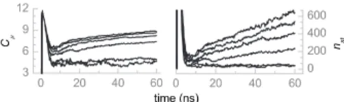
around the origin. The results for nr= 3 , 4 , 10, 20, 50 are presented in Fig.10. For nrⱕ4 the log2behavior in the tem-poral profile of the statistical complexity was completely de-stroyed and Cand the number of causal states saturated at a constant value. For higher nr the logarithmic behavior was retained, although the absolute values of Cwere somewhat lower than for the case of original data. Starting from the value of nrⱖ40, i.e., for the time scales longer than ⱖ1 ps, the value of statistical complexity remains unchanged. This result thus indicates that the statistical complexity at long time intervals共ⱖ1 ns兲 is completely defined by three orders of magnitude shorter dynamical patterns共ⱕ1 ps兲.
On the other hand, if the interval of the perturbations is less than the linear correlation time of 0.1 ps 共nrⱕ5兲 this destroys all longer-time correlations, making the signal simi-lar to the phase-shuffled surrogate characterized by very low values of C.
For disturbance intervals longer than the correlation time 共nr= 10, 20, 50兲 the number nst of the states is much less than that in the original data leading to reduced values of statistical complexity.
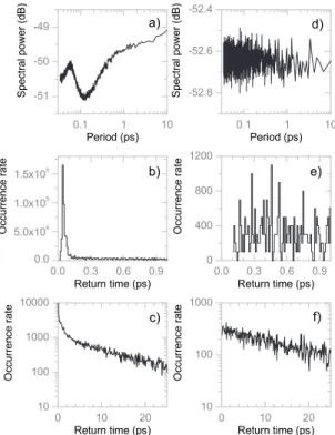
V. CAUSAL STATES CLUSTERING: “CORE” STATES To get a further insight into the link between the statistical complexity and the characteristic periods in the time series responsible for its high value, we analyzed the sets of causal states that constitute the ⑀ machine and, hence, define the statistical complexity through the distribution function of their occurrence rates P共⑀i兲. In order to distinguish between various time scales, we studied the time intervals between successive appearances of a causal state in the symbolic time series. For all the analyzed time series, we first identified the set of causal states and then plotted the histograms of recur-rence times共periods兲 for each of them. This analysis reveals that the causal states demonstrate a clear separation into two classes, which we will refer to as “core” states共those defined by short-time recurrences兲 and “noncore” states 共those with-out the well-defined characteristic time scale of recurrence兲. Core states are characterized by a clearly developed peak at the value of about 0.1 ps关see Fig.12共b兲兴, while the rest of the causal states are characterized by an exponential distri-bution of the recurrence times 关Figs. 12共e兲 and 12共f兲兴. In order to quantify the difference between the two classes, we introduce a dimensionless parameter G that characterizes the presence of the peak in the interval of the recurrencesⱕ1 ps 共compared to the interval 1 psⱕtⱕ2 ps兲,
G =max共h1兲 − m12 12
, 共4兲
where h1is the value of the recurrence time histogram in the time interval tⱕ1 ps, and m12,12 are the median and the FIG. 9. 共Color online兲 hQ values 共indicated on the right兲 for
SPCE共hQ= 0.69兲, TIP3P 共hQ= 0.78兲, and SPC 共hQ= 0.71兲 models of
water. The values for the SPC model at 275, 300, and 380 K are labeled 0.70, 0.71, and 0.76, respectively.
FIG. 10. Statistical complexity C and number of states nstfor
the temporal pattern-shuffled surrogate data with l = 9. From bottom to top, nr= 3 , 4 , 10, 20, 50, and the original data.
standard deviation values for the histogram in the interval 1 psⱕtⱕ2 ps. G can be used as a characteristic of each of the causal states. Its large value indicates high probability of the short-time recurrences, or, in other words, the quasiperi-odic nature of the corresponding causal state. The causal states characterized by a low value of G have “exponential” distribution of the return times and do not have pronounced low-order periodicity. In Fig.11we plot the scatter diagram representing the apparent clustering of the causal states into two classes with respect to the parameter G. The horizontal axis approximates the occurrence rate关or probability P共⑀i兲兴 of the causal states, i.e., for each of them we counted the number of its appearances in the symbolic time series and estimated the probability P共⑀i兲 by dividing it to the total length of the symbolic series.
Additional support to the observation of two qualitatively different classes of causal states is provided by Fourier analysis. For each of the causal states we generated a binary time series that contained “1” at those time moments where the given causal state was observed, and “0” elsewhere. By calculating the power spectra for the time series correspond-ing to the causal states we obtain an alternative indication of the difference between the core states and the rest of the set. Core states have a comparatively high level of spectral den-sity in the vicinity of the characteristic period of ⬇1 ps, whereas “noncore” states have a pronounced gap at this value, Figs. 12共a兲 and 12共d兲. This finding implies that the processes with characteristic time scales of⬇0.1 ps calcu-lated from the first zero of the correlation function as well as ⬇1 ps corresponding to the peak of the power spectrum are defined by the core causal states.
As for the phase-shuffled surrogate time series, the set of causal states is found to consist completely from the core states, i.e., the total number, probabilities, and even the sym-bolic sequences constituting the states approximately coin-cide with those of the core states of the ⑀ machine of the original signal. We can, therefore, conclude that the noncore causal states are the main reason for the high value of the statistical complexity in the MD signal.
The number of noncore states in the original signal grows approximately linearly with time. They are, therefore, re-sponsible for the phenomenon of the logarithmic growth of
C with time. The noncore states are defined by the long-time nonlinear correlations that are not captured by the 共lin-ear兲 autocorrelation analysis and completely absent in the surrogate signal.
Summarizing, the core states are always present, whatever the length of the time series or the location of the time win-dow on the time axis. The fact of the invariant presence of the core states indicates their key role in the formation of the power spectrum and correlation function. The rest of the ⑀ machine represents nontrivial, nonlinear, long-term processes that describe the way the system explores the phase space. For a molecular trajectory, the number of noncore states is high, indicating a perpetual process of exploring new areas in the phase space, whereas the absence of such states in the case of surrogate time series shows statistical stationarity of the latter and uniform phase-space coverage property of the surrogate trajectory.
VI. DISCUSSION AND CONCLUSIONS
The computational mechanics approach utilizing informa-tion theoretic concepts of the⑀machine and statistical com-plexity are used for describing the high-dimensional molecu-lar dynamics of an ensemble of 392 water molecules.
The problem of finding hidden regular patterns in a time series that appears to be a random process is addressed by the analysis of the phase-space filling property by an indi-vidual trajectory. The presence of patterns is judged by sig-FIG. 11. Clustering of the causal states for the hydrogen atom
velocity time series into core 共diamonds兲 and noncore 共triangles兲 classes. Parameter G is plotted vs occurrence rates of corresponding causal states.
FIG. 12. Power spectra关共a兲 and 共d兲兴 and histograms of recur-rence times关共b兲, 共c兲, 共e兲, and 共f兲兴 for typical causal states belonging to different types: a core state关共a兲–共c兲兴 and a noncore state 关共d兲–共f兲兴. The histograms on共c兲 and 共f兲 are zoomed and smoothed fragments of those shown in共b兲 and 共e兲. Spectra in 共a兲 and 共d兲 are the func-tions of inverse frequency.
nificant deviations from the uniform coverage of the phase space expected for the case of a random process.
Long-range memories present in the molecular dynamics simulations are detected and investigated by the means of statistical complexity analysis. It is shown that arbitrary long memories共much longer than one can expect from a spectral or correlation analysis兲 are present in the recorded time se-ries, manifesting themselves as groups of causal states in the velocity-defined phase space.
The noncore causal states change with the length of the analyzed molecular signal reflecting subtle differences in the statistics of the sequences of data points over time scales that are orders of magnitude longer than the common micrody-namics correlations. It should be stressed that these long-range correlations cannot be detected using the usual linear two-point statistics: the correlation function is essentially zero at all times for the data points spaced with intervals longer than a few picoseconds.
The time dependence of the statistical complexity value presumably comes from the fact that the microstate sampling is a slow process due to the extremely high value of the dimension of phase space. Since this time dependence origi-nates from the dimensionality of the phase space, the rate of the complexity change, hQ关Eq. 共3兲兴, should be an invariant for any microscopic observable 共provided that this observ-able is exhaustively sampled at these times兲. We have tested this hypothesis by comparing the complexity values obtained for the velocities of oxygen and hydrogen atoms to the time series of the instantaneous temperature Tinst. The result is presented in Fig.13where we plot the dependencies of C on time for one of the MD simulations. It is clear that the slopes of all the curves shown in Fig.13are indeed the same within numerical tolerance.
Finally, statistical complexity turns out to be a universal measure of dynamical structures present in the observed data. A comparison to surrogate data sets with broken dy-namical correlations supports the hypothesis that the patterns are not caused by the details of the computational procedure,
intrinsic statistical errors, or insufficient data, but by the complex dynamics of the system.
The rate of the temporal change in the statistical complex-ity value reflects the way the phase space of the system is explored共filled兲 by the trajectory. It can be conjectured that the exponent hQ represents a universal physical constant characterizing water, since it does not depend on the specific macroscopic observable analyzed, parameters of the system or simulation model, such as temperature, number of mol-ecules, or numerical model employed. It is also independent of the details of the data processing such as the choice of the phase-space partition used in the symbolization of the time series, the number of symbols, or the length of the histories used for reconstruction of the⑀machines. However, it does depend on the particular substance used in the simulations. For example, we have also investigated the case of a very different molecular system, liquid argon共Lennard-Jones liq-uid兲 and found significantly different values of hQcompared to the case of water. This will be the subject of future pub-lications.
The main results obtained in this paper by the analysis of the statistical complexity of a single MD trajectory共not an ensemble of independent trajectories兲 can be roughly sum-marized as follows:共i兲 over a long 共nanoseconds兲 time scale nontrivial structures in the probabilistic space 共far beyond the decay time of a conventional linear autocorrelation func-tion兲 are detected and analyzed; 共ii兲 the probabilistic 共causal兲 states demonstrate apparent clustering by the parameter G characterizing their periodicity 共recurrence times兲; 共iii兲 a measure is introduced that quantifies the growth of statistical complexity, i.e., the way the molecular system explores the phase space;共iv兲 the analysis of surrogate data reveals the absence of any significant causal states structures in the sur-rogate time series, thus indicating the dynamic nature of the temporal patterns that form causal states in the MD time series.
ACKNOWLEDGMENTS
This work was supported by Unilever and the European Commission共EC Contract No. 012835—EMBIO兲. The au-thors are grateful to an anonymous referee for careful read-ing of the manuscript and constructive comments that re-sulted in significant improvement of the paper.
APPENDIX: COMPUTATIONAL MECHANICS In nonlinear dynamics, common dynamic invariants such as dimensions, entropies, and Lyapunov exponents, are, in essence, simply sets of numbers used for characterizing the dynamics of the system. Obviously, it is hopeless to expect that one number or some small set of numbers can ad-equately describe a multidimensional complicated dynamical system such as water. In contrast, computational mechanics extracts all statistically significant information from the sig-nal at the same time achieving the maximal information compression 共see below兲, thus, providing a very desirable description of the dynamics.
FIG. 13. 共Color兲 hQ values共indicated on the right兲 for various
observables: black—the hydrogen velocity, red—the oxygen veloc-ity, and blue—the instantaneous temperature.
Computational mechanics analyzes symbolic dynamics, that is, a sequence of symbols, . . .s−2s−1s0s1s2. . ., from a finite alphabet of size K. All past si− and future si+ halves of bi-infinite symbolic sequences centered at times i are consid-ered. Two pasts s1−and s2− are defined equivalent if the con-ditional distributions over their futures P共兩s+兩s
1
−兲 and P共兩s+兩s 2 −兲 are equal. A causal state⑀共si−兲 is a set of all pasts equivalent to si−:⑀i⬅⑀共si−兲=兵: P共兩s+兩兲= P共兩s+兩si−兲其. At a given moment the system is at one of the causal states, and moves to the next one with the probability given by the transition matrix
Tij⬅ P共兩⑀j兩⑀i兲. The transition matrix determines the asymptotic causal state probabilities as its left eigenvector
P共⑀i兲T= P共⑀i兲, where 兺iP共⑀i兲=1. The collection of the causal
states together with the transition probabilities define an ⑀ machine.
It is proven关40兴 that the⑀machine is
共1兲 a sufficient statistic, that is, it contains the complete statistical information about the data;
共2兲 a minimal sufficient statistic, therefore the causal states cannot be subdivided into smaller states; and
共3兲 a unique minimal sufficient statistic, any other one simply relabels the same states.
The statistical complexity C= 0 is the information mea-sure of the size of the⑀machine that quantifies the amount of information about the past of the system that is needed to predict its future dynamics: C= H关P共⑀i兲兴, where H is the Shannon entropy of the distribution of a random variable X,
H关P共X兲兴⬅−兺XP共X兲log2P共X兲. ⑀ machines can be recon-structed from observed data using the CSSR algorithm de-scribed and implemented in Ref.关41兴.
Statistical complexity measures the informational content of the dynamics by searching and quantifying dynamical pat-terns in the signal. C= 0 both for completely random 共all values are independent兲 and completely ordered 共constant value兲 signals. For the intermediate cases the level of the order is estimated. However, in contrast to, for example, Fourier analysis, the shape of the patterns is not prescribed. Any patterns present are discovered.
For subsequences s−, s+of a finite length l the upper limit of the statistical complexity realized is when all of them are unique. In this case the number of causal states equals Kl with probabilities 1/Kl, where K is the alphabet size. Thus, the maximum possible value of the complexity is l log2K.
关1兴 A. M. Berezhkovskii and G. Sutmann, Phys. Rev. E 65, 060201共R兲 共2002兲.
关2兴 J. P. Crutchfield and K. Young, Phys. Rev. Lett. 63, 105 共1989兲.
关3兴 J. P. Crutchfield and K. Young, Entropy, Complexity, and Phys-ics of Information, SFI Studies in the Sciences of Complexity, VIII, edited by by W. Zurek共Addison-Wesley, Reading, Mas-sachusetts, 1990兲.
关4兴 J. P. Crutchfield, Physica D 75, 11 共1994兲.
关5兴 A. Cohen and I. Procaccia, Phys. Rev. A 31, 1872 共1985兲. 关6兴 V. Afraimovich and G. Zaslavsky, Chaos 13, 519 共2003兲. 关7兴 A. A. Brudno, Trans. Mosc. Math. Soc. 2, 127 共1983兲. 关8兴 S. Segre, Int. J. Theor. Phys. 43, 1371 共2004兲.
关9兴 V. Benci, C. Bonanno, S. Galatolo, G. Menconi, and M. Vir-gilio, Discrete Contin. Dyn. Syst., Ser. B 4, 935共2004兲. 关10兴 Coping with Chaos. Analysis of Chaotic Data and the
Exploi-tation of Chaotic Systems, edited by E. Ott, T. Sauer, and J. A. Yorke共John Wiley, New York, 1994兲.
关11兴 Dimensions and Entropies in Chaotic Systems, edited by G. M. Kress共Springer, New York, 1986兲.
关12兴 J. Cao, Phys. Rev. E 63, 041101 共2001兲.
关13兴 R. Cukier and J. Deutch, Phys. Rev. 177, 240 共1969兲. 关14兴 A. Rahman, Phys. Rev. 136, A405 共1964兲.
关15兴 M. G. Mazza, N. Giovambattista, F. W. Starr, and H. E. Stan-ley, Phys. Rev. Lett. 96, 057803共2006兲.
关16兴 P. Gaspard, M. E. Briggs, M. K. Francis, J. V. Sengers, R. W. Gammon, J. R. Dorfman, and R. V. Calabrese, Nature 共Lon-don兲 394, 865 共1998兲.
关17兴 C. P. Dettmann and E. G. D. Cohen, J. Stat. Phys. 101, 775 共2000兲.
关18兴 G. M. Zaslavsky, Phys. Rep. 371, 461 共2002兲.
关19兴 J. Theiler, S. Eubank, A. Longtin, B. Galdrikian, and J. Farmer, Physica D 58, 77共1992兲.
关20兴 J. Boon and S. Yip, Molecular Hydrodynamics 共McGraw-Hill, New York, 1980兲.
关21兴 U. Balucani and M. Zoppi, Dynamics of the Liquid State 共Ox-ford University Press, Ox共Ox-ford, 1994兲.
关22兴 B. M. Ladanyi and M. S. Skaf, Annu. Rev. Phys. Chem. 44, 335共1993兲.
关23兴 P. Grassberger and H. Kantz, Phys. Lett. A 113, 235 共1985兲. 关24兴 J. Plumecoq and M. Lefranc, Physica D 144, 231 共2000兲. 关25兴 M. A. Ricci, D. Rocca, G. Ruocco, and R. Vallauri, Phys. Rev.
A 40, 7226共1989兲.
关26兴 M. Wojcik and E. Clementi, J. Chem. Phys. 85, 6085 共1986兲. 关27兴 J. Teixeira, M. C. Bellissent-Funel, S. H. Chen, and B. Dorner,
Phys. Rev. Lett. 54, 2681共1985兲.
关28兴 H. J. C. Berendsen, J. Postma, W. van Gunsteren, and J. Her-mans, in Intermolecular Forces, edited by B. Pullman共D. Re-idel Publishing Company, Dordrecht, 1981兲, pp. 331–342. 关29兴 D. van der Spoel, E. Lindahl, B. Hess, G. Groenhof, A. E.
Mark, and H. J. C. Berendsen, J. Comput. Chem. 26, 1701 共2005兲.
关30兴 H. J. C. Berendsen, in Computer Simulations in Material Sci-ence, edited by M. Meyer and V. Pontikis共Kluwer, Dordrecht, 1991兲, pp. 139–155.
关31兴 W. G. Hoover, Phys. Rev. A 31, 1695 共1985兲.
关32兴 S. Wiggins, Introduction to Applied Nonlinear Dynamical Sys-tems and Chaos共Springer, New York, 1990兲.
关33兴 M. Buhl and M. B. Kennel, Phys. Rev. E 71, 046213 共2005兲. 关34兴 F. Takens, in Dynamical Systems and Turbulence, Lecture Notes in Mathematics 898, edited by D. A. Rand and L.-S. Young共Springer-Verlag, New York, 1981兲, pp. 366–381. 关35兴 A. C. Davison and D. V. Hinkley, Bootstrap Methods and their
Application, Cambridge Series on Statistical and Probabilistic Mathematics 共Cambridge University Press, Cambridge, En-gland, 1997兲.
关36兴 H. Kantz and T. Schreiber, Nonlinear Time Series Analysis 共Cambridge University Press, New York, 2003兲.
关37兴 P. Grassberger and I. Procaccia, Physica D 9, 189 共1983兲. 关38兴 H. D. I. Abarbanel, R. Brown, J. J. Sidorowich, and L. S.
Tsimring, Rev. Mod. Phys. 65, 1331共1993兲. 关39兴 G. Zaslavsky, Phys. Rep. 371, 461 共2002兲.
关40兴 C. R. Shalizi, K. L. Shalizi, and R. Haslinger, Phys. Rev. Lett.
93, 118701共2004兲.
关41兴 C. R. Shalizi, K. L. Shalizi, and R. Haslinger, in Uncertainty in Artificial Intelligence: Proceedings of the Twentieth Confer-ence, edited by M. Chickering and J. Halpern共AUAI Press, Arlington, Virginia, 2004兲, pp. 504–511; URL http://arxiv.org/ abs/cs.LG/0406011.