Crustal Structure in the Southern Kanto-Tokai
Region Derived from Tomographic Method for
Seismic Explosion Survey
Zhixin Zhao,1,* Ryuji Kubota,1 Fumio Suzuki,2 and Susumu Iizuka3
1 Kawasaki Geological Engineering Co., Ltd., 6-24-10 Minami-Oi, Shinagawa-ku, Tokyo 140, Japan
2 Nippon Geophysical Prospecting Co., Ltd., 2-2-12
Nakamagome, Ohta-ku, Tokyo 143, Japan 3
Department of Marine Mineral Resources, School of Marine Science and Technology, Tokai University,
Shimizu 424, Japan
The detailed P-wave velocity structure of the crust in the southern Kanto-Tokai region was analyzed using the tomographic method for seismic refraction survey in this paper. A total of 332 P-wave arrival times received from 13 seismic explosion surveys were used in the analysis. The results indicate that analyses of travel-time curves are probably useful for the evaluation of inverted structures. The lateral heterogeneity of the velocity structure is obviously related to tectonics. The crust in the eastern region is thinner than that in the western region. The Conrad discontinuity obviously fluctuates. The granitic layer is thinner beneath the oceanic region to the east of Oshima. The layer becomes about 16 km thick beneath Suruga Bay. The Conrad discontinuity drops nearly 17 km in depth beneath Suruga Bay, and velocity is relatively low there. The Conrad discontinuity rises 6 km beneath MTL and its vicinity. The Moho discontinuity is located at a depth of around 34 km beneath the region to the west of ISTL and roughly coincides with the upper boundary of the seismic zone due to subduction of the Philippine Sea Plate under the Eurasian Plate. It becomes shallow across the Suruga trough toward the eastern region. The discontinuity is located about 27 km in depth beneath the oceanic region east of Oshima.
1. Introduction
The southern Kanto-Tokai region is one of the most complicated structural regions in Japan. The Nankai, Suruga, and Sagami troughs in the region are regarded as the northern boundary of the Philippine Sea Plate. Major geological tectonic lines such as the Median tectonic line (MTL), the Akaishi tectonic line (ATL), the Itoigawa-Shizuoka tectonic line (ISTL), etc., pass through this region as shown in Fig. I. Moreover, the
Received May 23, 1997; Accepted January 7, 1998 * To whom correspondence should be addressed .
Fig. I. Locations of shot and observation sites and major tectonic features in the southern Kanto-Tokai region, Japan. Reciprocal triangle, shot site; open circle, observation site. S1 (Neo, Gifu) and S3 (off Boso) are two end-points of the studied profile. MTL, Median tectonic line; ISTL, Itoigawa-Shizuoka tectonic line; ATL, Akaishi tectonic line.
volcanic front to the east of Izu Peninsula extends along the north-south direction,
where the Fuji and Hakone volcanoes lie. The southern Kanto-Tokai region is also one
of the most seismically active zones in Japan. The nature of the complicated geological
tectonics and seismic activity, as mentioned above, in the southern Kanto-Tokai region
has been extensively investigated by seismic and other geophysical methods for decades.
Bodri et al. (1991) and Bodri and Iizuka (1993) suggested significant correlation among
the heat flow, cutoff depth of earthquakes and depths to the Conrad and Moho
dis-continuities. Studies on the velocity structure in this region have also been carried out
as a part of earthquake prediction research programs (e.g., Yoshii et al., 1986).
The velocity structures of crust and upper mantle have been widely studied through
explosion seismic refraction surveys in the region. Many results obtained from the time
term technique have been reported in the last 30 years (Yoshii, 1994). Asano et al.
(1985) studied the velocity structure along a north-south directional profile in the Izu
Peninsula and its vicinity located in the northern part of the Philippine Sea Plate. The
result suggested that the crust becomes thin toward the southern portion. The
struc-tures of crust and upper mantle of the Inabu (137•‹31'E, 35•‹13'N, in Gifu Prefecture)-
Oshima profile and the Neo (in Gifu Prefecture) (S1)-Izu-off Boso (S3) profile (in
Fig. 1) were studied by Ikami (1978) and Suzuki (1987), respectively through analyzing
the travel times from explosion seismic observations mainly using Aoki's method (Aoki,
1971). Both results confirmed that a thrusting to the east at the MTL reached several
kilometers. An explosion seismic refraction survey can generally study detailed
structures. With respect to the analysis of wave propagation in a complicated geological
structure, it is better to use the highly accurate tomographic method developed in recent
years. Methods of tomographic inversion of seismic travel time residuals are now
established and widely used in the technique for imaging the earth's interior. Many results from the tomographic method have already been reported (Hirahara, 1990). The results of seismic tomography using explosion seismic observations were also applied in a study on tectonics (Mochizuki et al., 1997). These results have helped and improved our understanding of geophysical and geological processes in the earth. Ishida and Hasemi (1988) studied three-dimensional fine velocity structure and hypocentral dis-tribution of earthquakes beneath the Kanto-Tokai district by tomographic inversion
using the observed travel times of earthquakes. The obtained results were successfully employed in the interpretation of plate tectonics for movements of the Pacific and Philippine Sea Plates in the Kanto region.
In this analysis, the tomographic method for seismic refraction survey was em-ployed to invert the velocity structures of crust and uppermost mantle in the southern Kanto-Tokai region using the observed travel times from explosion seismic surveys. The structures will be analyzed starting from different initial models using the tomo-graphic method. The travel-time curves were used to analyze the crustal structure. The relationship between the structure of the crust in the region and local seismicity is discussed.
2. Data and Method
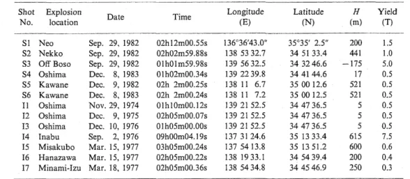
The data of observed travel times used in the tomographic analysis were obtained from thirteen explosions. Table 1 lists the databases of the thirteen explosions. The shot numbers prefixed with the letter "S" in Table 1 means that the data are selected from the report by Suzuki (1987) and Den et al. (1985) (report 1). The prefixed letter "I" means that the data are from the report by Ikami (1978) (report 2). Locations of 13 shots and more than 100 observation stations both on land and on the sea floor are shown in Fig. 1. Fundamental data such as the origin times and the locations of stations
Table 1. Data on explosion experiments and quarry blasts.
S-shot No., reference from Suzuki, 1987; I-shot No., reference from Ikami, 1978. Vol. 45, No. 6, 1997
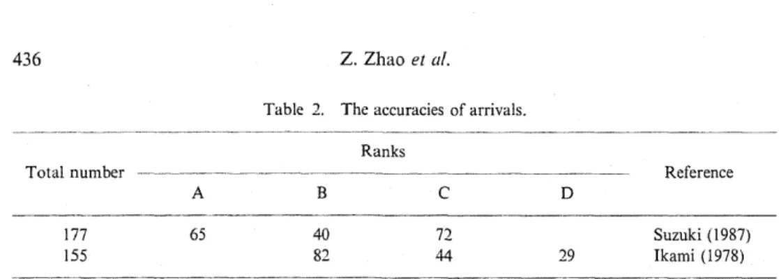
Table 2. The accuracies of arrivals.
Rank A, B, C, and D denote the accuracies of onset times within 0.01, 0.05, 0.1, and 0.2 s, respectively.
were reported in the original reports (Den et al., 1985; Suzuki, 1987; Ikami, 1978). The 332 first arrivals of P waves are employed in the tomographic analysis.
The arrival times from report 1 were generated by 6 explosion experiments and data from a total of 75 observation stations in the Neo-Izu Peninsula-off Boso profile on September 29, 1982, December 9, 1982, and December 9, 1983. The station intervals are about 5 km, and the survey line is about 330 km between Neo in Gifu Prefecture (S1) and off-Boso (S3) along the east-west direction. Seismographs with natural frequencies of 2 or 3.5 Hz were used for the observations. Most of the seismograms obtained are of good quality. The observation accuracies of arrival times were within 0.1 s for both the first and later phases. A total of 177 arrivals were selected from the above reports to be used in this analysis. Table 2 lists the observation accuracies of arrival times. The number of arrivals having accuracies within 0.01, 0.05, and 0.1 s were 65, 40, and 72, respectively.
Other travel times from report 2 were observed by the sets of 7 shots as shown in Table 1 and about 50 observation stations. Some of the explosion experiments were carried out by the Geological Survey of Japan (GSJ). Seismographs having a vertical component with a natural frequency of 1 Hz were used in the explosion observations. Some data of explosion surveys from GSJ were employed to detect the secular changes of P-wave velocity in the southern Kanto district. A part of them was employed to investigate the shallow crustal structure in western Shizuoka (Ito et al., 1977). A total of 155 arrivals selected from the latter report were also used in the analysis. The sampling rate is 0.01 s. The observation accuracies of the arrivals are shown in Table 2. The number of events having accuracy within 0.05, 0.1, and 0.2 s were 82, 44, and 29, respectively.
In this analysis, the pseudo-bending method, a fast algorithm for two-point ray tracing (Urn and Thurber, 1987) was used in determining the ray path and calculating travel times. The method can find an accurate ray path in a full three-dimensional velocity structure even where lateral variations in velocity are severe. In addition, the method provides some computational advantage because the direct minimization of travel time replaces solving the ray equation. The conjugate gradient (CG) algorithm (Hestenes and Stiefel, 1952) was employed to solve the discrete linearized equation for the travel-time differences between the computed and observed information in the in-version because of its fast and accurate advantages of calculation. A full-index scheme
(Scales, 1987) was also used in the calculation of sparse matrices because the coefficient matrix of the linearized equation for differences in travel times is sparse.
3. Analysis and Results
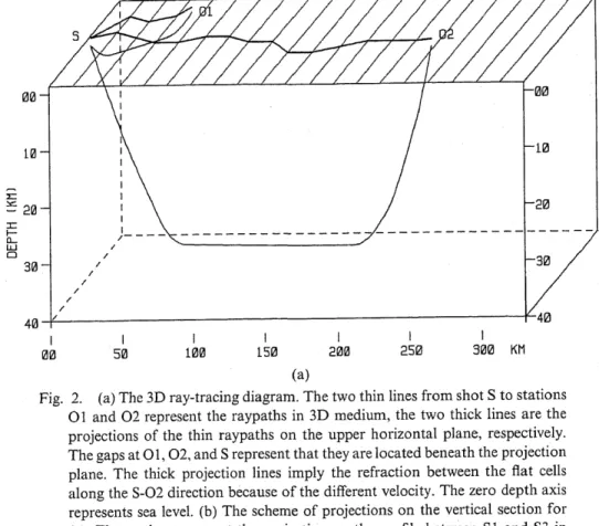
The observation stations and shots with different elevations set on the ground surface and on the sea floor do not exactly align along the profile between Si and S3 as shown in Fig. 1. They extend for about 50 km in width in the direction perpendicular to the profile line. Therefore, ray-tracing by the pseudo-bending algorithm is necessary in the three-dimensional (3D) medium to obtain an accurate theoretical travel time. The velocity, however, is assumed to be unvarying along the direction perpendicular to the profile line in the analysis. Figure 2(a) illustrates 3D ray-tracing from the pseudo-bending method. The two thin lines from shot S to stations O1 and O2 represent the raypaths in 3D medium. The two thick lines on the upper horizontal plane are the projections of the corresponding thin raypaths in 3D cubic medium. These thick lines (projections of raypaths) mean the fraction from mesh to mesh because of the different
(a)
Fig. 2. (a) The 3D ray-tracing diagram. The two thin lines from shot S to stations O 1 and O2 represent the raypaths in 3D medium, the two thick lines are the projections of the thin raypaths on the upper horizontal plane, respectively. The gaps at O1, O2, and S represent that they are located beneath the projection plane. The thick projection lines imply the refraction between the flat cells along the S-O2 direction because of the different velocity. The zero depth axis represents sea level. (b) The scheme of projections on the vertical section for (a). The meshes represent the projection on the profile between Si and S3 in Fig. 1 for the divided cells of medium in (a). The 2D raypaths from S to O1 and 02 are the projections on the profile for 3D raypaths formed by the straight-line segments between the two points that the corresponding raypaths in (a) intersect in the boundary planes of cells.
Fig. 2(b)
velocities in the flat meshes along the S1-S3 direction.
The velocity structure in the profile between S1 and S3 was analyzed as a two-dimensional (2D) problem. Figure 2(b) shows the scheme of mesh division for the profile between Si and S3 in Fig. 1. The 240 velocity cells cover the whole profile in the analysis. The different vertical sizes of cells were defined on the basis of the velocity structure to reduce the number of cells in the computation. The thickness of the uppermost layer is 4 km including a 1.5 km elevation to suit the observation stations and/or shots set in the mountains. The thickness of each layer is 2.5 km from the depth of 2.5 to 20 km and 5 km from the depth of 20 to 35 km. The horizontal length of a cell is selected as 16.5 km. A unique value of velocity was adopted in the cell. The velocity at any point in the cell can be interpolated to suit ray-tracing by the pseudo-bending algorithm. The 2D raypaths from S to O1 and O2 in Fig. 2(b) are projections on the profile for the 3D raypaths formed by the straight-line segments between the two points which the corresponding arc raypath (in Fig. 2(a)) intersects the boundary planes of the cubic cell. Travel times for both the line segment raypath and arc raypath directly obtained from the bending method (Fig. 2(a)) were calculated in the analysis. The former better approximates the observed travel time generally. We prefer the travel time of the 3D straight-line segment ray rather than that of the arc ray in the inversion. Some cells with no illumination (or terminal small illumination) might appear because the ray did not pass through (or grazed) the cells in the ray tracing process ('unknown' portion in Figs. 4, 5, and 10). So the column elimination technique was applied in the inversion of perturbation vector slowness.
The inversion was progressively implemented by iteration. The perturbations of slowness obtained from the discrete linearized equation were used to modify the last model of velocity, then ray-tracing was carried out again in the new structure of velocity, and so on.
(a) (b)
(c)
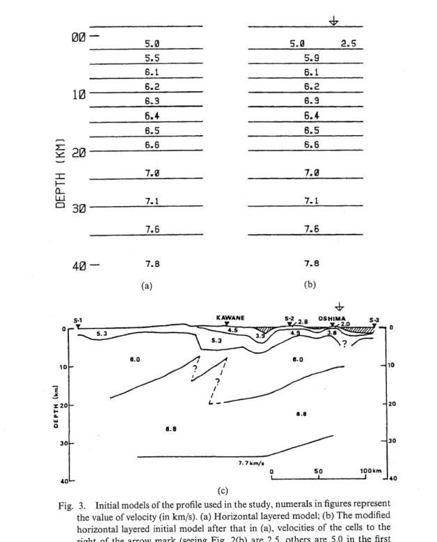
Fig. 3. Initial models of the profile used in the study, numerals in figures represent the value of velocity (in km/s). (a) Horizontal layered model; (b) The modified horizontal layered initial model after that in (a), velocities of the cells to the right of the arrow mark (seeing Fig. 2(b) are 2.5, others are 5.0 in the first layer. The location of arrow mark corresponds to that in Figs. 2(b) and 3(c); (c) 2D velocity structure in the Tokai region by Suzuki (1987).
3.1 Results of analysis
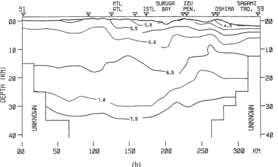
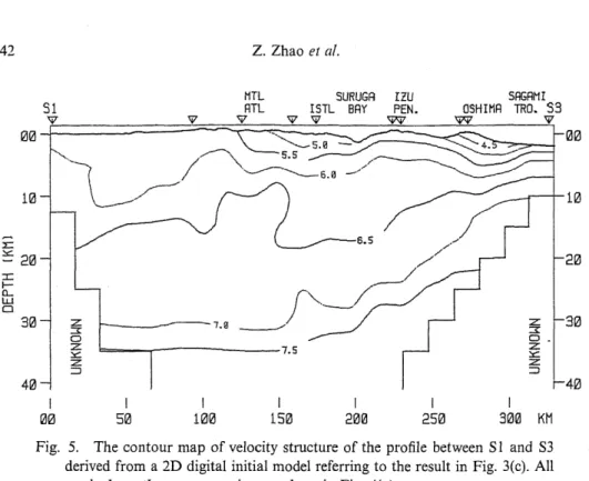
The various initial models, as shown in Fig. 3, were employed to obtain the velocity structure of the profile between S1 and S3. Some differences related to the initial model appear in the results as shown below, although the patterns of structure are similar to each other. The inversion result with the smallest standard deviation of travel-time residuals between the observed and calculated one for the horizontally layered initial model (in Fig. 3(a)), 0.231 s, was obtained at the tenth iteration. Figure 4(a) shows the inverted structure by using contours with a velocity interval of 0.5 km/s. The lines of 5.5, 6.5, and 7.5 km/s are drawn as thick lines. The east area near shot S3 is the ocean region in Fig. 1. In Fig. 3(b), we change velocities in the three cells from the east oceanic end in the first layer (east to the arrow mark in Fig. 2(b), Fig. 3(b) and (c)) to 2.5 km/s. The velocity 5.5 km/s in Fig. 3(a) was also changed by 5.9 km/s for the second layer of the model in Fig. 3(b). The velocities in other layers are the same for both Fig. 3(a) and (b). Figure 4(b) shows the inverted structure with the smallest standard deviation of travel-time residuals for the initial model in Fig. 3(b), 0.231 s, using the same manner as that for Fig. 4(a). The inverted structures in Fig. 4(a) and (b) have similar characteristics. Figure 5 shows the velocity structure obtained from the 2D digital initial model referring to the result by Suzuki (1987) in Fig. 3(c) using the same technique as for Fig, 4. The inverted result with the smallest standard deviation of travel-time residuals for the initial model in Fig. 3(c), 0.230 s, was obtained at the ninth iteration. Figure 6 shows the 3D ray-tracing result for 332 seismic rays obtained from the pseudo-bending algorithm under the structure in Fig. 5 and the locations of shots in the southern Kanto-Tokai region. In the calculations for the three initial models above, both travel times for the arc raypaths, like those shown in Fig. 6, and the 3D seismic raypaths formed by the straight-line segments between the two points, which the corresponding
(a)
(b)
Fig. 4. (a) The velocity structure in the profile between S1 and S3 in Fig. 1 derived from the horizontal layered initial model of Fig. 3(a). The numerals sets in contours represent the value of velocity (in km/s). The top thick line represents the elevation of topography. The meanings of the abridged letters at the top of the figure are the same as those in Fig. 1. The reciprocal triangles at the top of the figure represent the shot sites. The 'UNKNOWN' portions without isopleth line in the lower right and left corners are no illumination regions. (b) The contour map of velocity structure of the profile between S1 and S3 derived from the modified layered initial model in Fig. 3(b). All marks have the same meanings as those in (a).
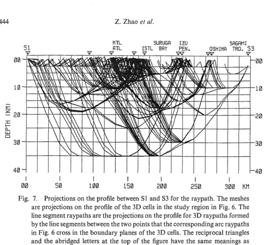
arc raypaths (in Fig. 6) intersect the boundary planes of cubic cells, were calculated. Figure 7 shows the projections on the profile between S1 and S3 for the 3D seismic raypaths formed by the segments. The average standard deviations of travel-time residuals in the case of the arc raypath (in Fig. 6) were larger than those in the case of segment raypath usually. The theoretical travel times with high accuracy for the 3D seismic raypaths formed by the straight-line segments were employed into the inversions of the three models.
In order to evaluate the structures as shown in Fig. 4(a) (obtained from initial model of Fig. 3(a)), 4(b) (obtained from initial model of Fig. 3(b)) and Fig. 5 (obtained from the 2D digital initial model in Fig. 3(c)), both observed and calculated arrival times under the three models were analyzed further. The results for the explosion experiment in Neo (shot S1 in Table 1), Nekko (S2 in Table 1) and Off-Boso (S3 in Table 1) are expounded in detail because the explosions have a long survey distance and many observation stations. The standard deviations of the difference between the observed and calculated arrivals under the structure result in Fig. 4(b) are 0.149, 0.208,
Fig. 5. The contour map of velocity structure of the profile between S1 and S3 derived from a 2D digital initial model referring to the result in Fig. 3(c). All marks have the same meanings as those in Fig. 4(a).
and 0.278 for S1, S2, and S3 cases, respectively. The corresponding parameters under the structure model in Fig. 4(a) are 0.167, 0.232, and 0.302, respectively. It can be seen that the standard deviation of differences between observed travel times and calculated travel times are smaller in the case for the initial model in Fig. 3(b) than those for the initial model shown in Fig. 3(a). As an example, Fig. 8 gives the observed and calculated travel-time curves from the structure in Fig. 4(b) for S1, S2, and S3. Similarly, Fig. 9 shows the observed and theoretical travel-time curves for S1, S2, and S3 shots, cal-culated under the structure in Fig. 5. The standard deviations of the differences between the observed and calculated travel times are 0.169, 0.254, and 0.270 for S1, S2, and S3 cases, respectively. A discontinuity of velocity appears at the epicentral distance of about 135 km for the S3 case in Figs. 8 and 9. The velocity calculated from the arrivals with a distance greater than 135 km approximates 7.5 km/s, which is equivalent to that of head wave Pn refracted from the Moho discontinuity. The velocity from the travel times less than 135 km approximates 6.2 km/s, which is equivalent to the velocity of P wave from the granitic layer.
3.2 Characteristics of the velocity structure
The obtained characteristics of velocity structure starting from the initial layered model in Fig. 3(a) and model in Fig. 3(b), as mentioned above, are very similar mutually as shown in Fig. 4(a) and (b). The velocity structure characterizes the lateral hetero-geneity. The surface layer of crust with a velocity of less than 5.5 km/s appears mainly in the region to the east of the MTL, most of which are sea regions, and this layer is very thin. The layer between the contours of 5.5 and 6.5 km/s can be regarded as the
Fig. 6. The 3D ray-tracing result. The upper figure shows the geographic dis-tribution of all shots in Table 1 (reciprocal triangles between S1 and S3 in Fig. 1) in the study region, and the lower figure shows a 3D ray-tracing ob-tained from the pseudo-bending algorithm under the structure in Fig. 5.
granitic layer. The boundaries of the layer fluctuate, especially that of 6.5 km/s, called Conrad discontinuity, changes. The granitic layer beneath the ocean region to the east of Oshima is about 7 km. The Conrad discontinuity (contour of 6.5 km/s) deepens to near 19 km beneath Suruga Bay. The granitic layer thickens to greater than 15 km beneath Suruga Bay. The layer thins to about 10 km beneath ATL and MTL and its eastern vicinity because the Conrad discontinuity rises by about 5 km beneath the region between ISTL and MTL. The layer becomes thicker and is about 13 km in the western region to MTL.
The lower layer between the isopleth of 6.5 km/s and that of 7.5 km/s can be taken as the basaltic layer in the crust in Fig. 4(a) and (b). The lower interface of the basaltic layer (i.e., the Moho discontinuity) is located at a depth of about 34 km beneath the western region to ISTL. The thickest portion of the basaltic layer is about 22 km beneath the MTL because the Conrad discontinuity rises as mentioned previously. Then, the Moho discontinuity rises from the region beneath Suruga Bay to the east, and becomes about 27 km deep beneath Oshima Island and its eastern vicinity.
Fig. 7. Projections on the profile between S1 and S3 for the raypath. The meshes are projections on the profile of the 3D cells in the study region in Fig. 6. The line segment raypaths are the projections on the profile for 3D raypaths formed by the line segments between the two points that the corresponding arc raypaths in Fig. 6 cross in the boundary planes of the 3D cells. The reciprocal triangles and the abridged letters at the top of the figure have the same meanings as those in Fig. 1.
The velocity structure in Fig. 5, from the 2D digital initial model, obviously characterizes the lateral heterogeneity, and some properties are similar to the results in Fig. 4. The thin layer with velocity less than 5.5 km/s appears only in the region to the east of MTL. The layer with the velocity of 4.5 km/s appears in the oceanic region to the east of Oshima. The layer between the contour of 5.5 and 6.5 km/s, regarded as the granitic one, extends laterally over the whole region. The granitic layer beneath the ocean region to the east of Oshima is the thinnest portion in the whole layer, less than 5 km. It thickens gradually from the eastern to western regions, the lower boundary drops to a depth of about 10 km beneath the Izu Peninsula and obtains a thickness of near 15 km beneath Suruga Bay and ISTL. The layer thins suddenly to about 5 km beneath ATL, MTL and its eastern vicinity because the Conrad discontinuity sharply rises by about 9 km there. The layer becomes about 15 km thick in the western region to MTL. The Conrad discontinuity fluctuates more severely than the cases in Fig. 4(a) and (b).
The basaltic layer is thicker than the above granitic layer in Fig. 5. The contour of 7.5 km/s for the basaltic layer, called the Moho discontinuity, is smoothly located at a depth of about 35 km beneath the western region to ISTL. The thickest portion of the basaltic layer is about 25 km beneath MTL. Then, the Moho discontinuity rises from the region beneath ISTL and Suruga Bay to the east, almost parallel with the
Fig. 8. The travel-time curves for the explosions at Neo (S1), Nekko (S2), and off-Boso (S3, in Table 1). The open circles represent observed reduced travel times and crosses represent reduced travel times calculated under the structure in Fig. 4(b). The ordinate is the reduced travel time (s), and the abscissa is the epicentral distance (km).
Fig. 9. The travel-time curves for the explosions at Neo (S1), Nekko (S2), and off-Boso (S3). The open circles represent observed reduced travel times and the crosses represent reduced travel times calculated for the structure shown in Fig. 5. The other legend has the same meaning as that in Fig. 8.
Conrad discontinuity, and becomes about 22 km deep beneath Oshima Island and its eastern vicinity. The western portion of the basaltic layer is thicker than the eastern portion.
The crustal structure in the south Kanto-Tokai region was analyzed using the tomographic method for seismic refraction. Three tests conducted by changing the initial model indicate that the pattern of crustal structure in the region is stable as mentioned above. The structures in Fig. 4(a), obtained from the layered initial model in Fig. 3(a), and that in Fig. 4(b), from the modified layered model in Fig. 3(b), are similar to the result in Fig. 5 from the 2D digital initial model in Fig. 3(c). The depths of the Moho and Conrad discontinuities in the western region in Fig. 5 approach those in Fig. 4(a) and (b). The rise of the Conrad discontinuity beneath MTL and its eastern vicinity in Fig. 5 can also be seen in Fig. 4(a) and (b) although the rise in Fig. 5 is higher than those in Fig. 4(a) and (b). It can obviously be seen that the Conrad discontinuity beneath Suruga Bay is low in all three velocity structures shown in Figs. 4(a), (b), and 5. The thickness of the granitic and basaltic layers beneath the regions to the east of Suruga Bay (about 135 km away from shot S3) in Fig. 5 differs from those in Fig. 4(a) and (b) somewhat. Few stations were set up in Suruga Bay and the eastern oceanic region (see Fig. 1 or 7) because of geographic limitations. Such lack of records causes the different inversion results, especially in the case of the complicated geological structure. Namely, the inverted velocity structure probably depends on the initial model in the eastern ocean region in the present case from the lack of recorded data. Perhaps the lack of records is the reason that the structures beneath the area to the east of
Suruga Bay in Fig. 5 differ from those in Fig. 4(a) and (b). The travel-time curves less than 135 km show that the fitting status between observed and calculated arrivals for
S3 in Fig. 8, differs from that in Fig. 9, the difference for Si status between two figures, however, is not obvious. The results of this paper suggest that the analyses of travel-time curves are probably useful in the evaluation of the structures from different starting model under such circumstances.
The new structure has been synthesized by averaging the results in Figs. 4(a), (b), and 5, and is shown in Fig. 10 to understand characteristics of the velocity structure in the region. The theoretical travel times were directly calculated under the synthesized model in Fig. 10. Figure 11 shows the observed and theoretical travel-time curves for S1, S2, and S3 shots. The standard deviations of the travel-time residuals are 0.239, 0.252, 0.344 for S1, S2, and S3 cases, respectively. It can be seen that the fitting status between the observed and three theoretical travel-time curves in Fig. 11 are well on overall.
4. Discussion
The south Kanto-Tokai region is one of the most tectonically and seismically active regions in the Japanese Islands. The Philippine Sea Plate subducts beneath the Eurasian Plate at the Nankai, Suruga, and Sagami troughs. The results obtained indicate that characteristics of the crustal velocity structure are probably related to the tectonics in the region. In order to investigate the relationship between tectonics and the crustal structure, we analyzed seismic activity (Ishikawa et al., 1985; Ishikawa, 1986) in the
Fig. 10. A contour map of the synthesized velocity structure of the profile be-tween S1 and S3 by averaging the three velocity structures shown in Figs. 4(a), (b), and 5. All marks have the same meanings as those in Fig. 4(a).
region using an earthquake catalogue, with high accuracy during the period between
1983 and 1994, from the Japan Meteorological Agency. Figure 12 shows the depth
distribution of earthquakes with the crustal structure of Fig. 10 along the profile. The
lateral heterogeneity of crustal velocity is obviously related to the distribution of the
hypocenters.
The earthquake distribution can be divided into two layers beneath MTL and ATL
(about 138•‹E), and the region to the west of them in Fig. 12(b). The events in the upper
layer at the depth between 5 and 20 km are located in the upper crust of the Eurasian
Plate. The contour of 6.5 km/s, called the Conrad discontinuity, approximates to the
lower boundary of the upper seismic layer beneath the region to the west of MTL
except for the region under MTL. The events that occurred below the contour of
6.5 km/s under MTL and ATL seem to be related to a rise of about 30 km wide of the
basaltic layer, which may be caused by an upward thrust movement at MTL. The high
velocity region is also a seismically active portion compared with the two sides. The
lower crust is practically aseismic, this result is similar to the results obtained by Bodri
et al. (1991), and Bodri and Iizuka (1993). The lower seismic layer, around 40 km in
depth (Fig. 12(b)) and about 20 km thick, is composed by the events due to the subduction
from the Philippine Sea Plate. The Moho discontinuity (contour 7.5 km/s) obtained in
this analysis approaches the upper boundary of this seismic layer beneath MTL and
ATL, and the region to the west of them.
The Conrad discontinuity, about 40 km wide beneath Suruga Bay, is 6 km lower
than both sides, approaching nearly 17 km in depth in Figs. 10 and 12(b). It is a
low-velocity region. Such characteristics of variation are consistent with the low-velocity
Fig. 11. The travel-time curves for the explosions at Neo (S1), Nekko (S2), and off-Bolo (S3). The open circles represent observed reduced travel times and the crosses represent reduced travel times calculated for the structure shown in Fig. 10. The other legend has the same meaning as that in Fig. 8.
(a)
(b)
Fig. 12. (a) Seismicity (M•¬2.5, 1983-1994) in the southern Kanto-Tokai region. (b) The comparison for depth distribution of earthquakes in the profile between A in Fig. 12(a) (S1) and B in Fig. 12(a) (S3), and the velocity structure shown in Fig. 10.
region at 16 km in depth from the earthquake data reported by Ishida and Hasemi (1988) and Ishida (1992). The low-velocity region is located in the upper portion of the subduction seismic zone dipping from Suruga Bay to the area beneath the region east of MTL (Fig. 12(b)). The granitic layer is thin beneath the oceanic region to the east of Oshima in Fig. 10. The depth of the Conrad discontinuity is around 10 km in Fig. 10 beneath that place. This is consistent with the depth obtained by Furumoto et al. (1989). The crust thickness is approximately 28 km beneath Oshima, being slightly less than the result of 30 km by Ishida (1992). The depths of earthquakes are almost less than that of the Moho discontinuity beneath the region to the east of Suruga Bay except the events occurring in the subduction zone of the Pacific Plate beneath the Sagami trough (S3 in Fig. 12(b)).
The Moho discontinuity is located at a depth of around 34 km beneath the region to the west of MTL in Fig. 10. It rises to 28 km to the east of the Suruga trough. The Philippine Sea Plate subducts beneath the Eurasian Plate into the western northwest-eastern southeast direction along the Suruga trough. The seismic zone dips toward the west from Suruga Bay to the area beneath the region east of MTL in Fig. 12(b). The depth variation of the Moho discontinuity crossing over the Suruga trough may imply that the crust in the region of the Philippine Sea Plate to the east of the Suruga trough is thinner than the crust in the region of the Eurasian Plate west of the trough. 5. Conclusions
The crustal structure of the profile between Neo (S1) in Gifu Prefecture and the off-Boso (S3) in the southern Kanto-Tokai region was analyzed using the P-wave tomographic method for seismic refraction survey in this paper. The results suggest that the lateral heterogeneity of the velocity structure is related to the tectonics and seismic activity in the region.
1. The crust in the eastern oceanic region is thinner than that in the western region.
2. The Conrad discontinuity (or the basaltic layer) rises by about 5 km beneath the Median tectonic line (MTL) or the Akaishi tectonic line (ATL) compared with the two sides. The raised portion of the basaltic layer coincides with a seismically active zone. It implies that the tectonic movement with upward thrust component has occurred beneath MTL and/or ATL.
3. The Conrad discontinuity beneath the Suruga trough exists at the depth of about 17 km and is deeper than both sides. A low velocity region appears beneath the trough.
4. The Moho discontinuity is located at around 34 km beneath the western part and coincides with the upper boundary of the seismic zone due to the subduction of the Philippine Sea Plate under the Eurasian Plate. Discontinuity becomes shallower across the Suruga trough toward the eastern region and it is about 27 km deep beneath Oshima.
5. The analysis of travel-time curves may be useful in the evaluation of the velocity structure obtained from the tomographic method under such circumstances.
The authors are very grateful to Dr. Y. Ishikawa, the Meteorological Research Institute for the Seis-PC program and his kind help. Two anonymous reviewers are acknowledged for their extensive reviews of this manuscript.
REFERENCES
Aoki, H., A least squares method in the analysis of crustal structure, in Islandarc and Marginal Sea, pp. 83-92, Tokai University Press, Tokyo, 1971 (in Japanese).
Asano, S., K. Wada, T. Yoshii, M. Hayakawa, Y. Misawa, T. Moriya, T. Kanazawa, H. Murakami, F. Suzuki, R. Kubota, and K. Suyehiro, Crustal structure in the northern part of the Philippine Sea Plate as derived from seismic observations of Hatoyama-off Izu Peninsula explosions, J. Phys. Earth, 33, 173-189, 1985.
Bodri, B. and S. Iizuka, Earthquake cutoff depth as a possible geothermometer-applications to central Japan, Tectonophysics, 225, 63-78, 1993.
Bodri, B., S. Iizuka, and M. Hayakawa, Geothermal and rheological implications of intra-continental earthquakes beneath the Kanto-Tokai region, Central Japan, Tectonophysics, 194, 337-347, 1991.
Den, N., S. Asano, T. Kanazawa, Y. Misawa, S. Iizuka, T. Yoshii, F. Suzuki, A. Ikami, Y. Sasaki, T. Moriya, and R. Kubota, Explosion seismic observation in the Neo-Izu Peninsula-off Boso profile, Bull. Inst. Oceanic Res. Develop., Tokai Univ., 7, 77-91, 1985 (in Japanese with English abstract).
Furumoto, M., T. Kunitomo, and H. Inoue, Depth contour maps of the discontinuity surfaces of the crust in and around the south Fossa Magna, Mod Geol., 14, 35-46, 1989.
Hestenes, M. and E. Stiefel, Methods of conjugate gradients for solving linear systems, Nat. Bur. Stand. J. Res., 49, 409-436, 1952.
Hirahara, K., Inversion method of body wave data for three-dimensional earth structure, Zisin, Ser. 2, 43, 291-306, 1990 (in Japanese with English abstract).
Ikami, A., Crustal structure in Shizuoka district, central Japan as derived from explosion seismic observations, J. Phys. Earth, 26, 299-331, 1978.
Ishida, M., Geometry and relative motion of the Philippine Sea Plate and Pacific Plate beneath the Kanto-Tokai district, Japan, J. Geophys. Res., 97, 489-513, 1992.
Ishida, M. and A. Hasemi, Three-dimensional fine velocity structure and hypocentral distribution of earthquakes beneath the Kanto-Tokai district, Japan, J. Geophys. Res., 93, 2076-2094,
1988.
Ishikawa, Y., The outline of the revised edition of SEIS-PC, Geol. Data Process, 11, 65-74, 1986 (in Japanese).
Ishikawa, Y., K. Matsumura, H. Yokoyama, and Y. Matsumoto, SEIS-PC-its outline, Geol. Data Process, 10, 19-34, 1985 (in Japanese).
Ito, K., I. Ichikawa, I. Hasegawa, T. Kakimi, S. Iizuka, M. Takahashi, E. Yamamoto, and T. Nishikata, Crustal structure in western Shizuoka Prefecture, Abstr. Ann. Meet., Seismol. Soc. Jpn., 2, 124, 1977 (in Japanese).
Mochizuki, K., J. Kasahara, T. Sato, M. Shinohara, and N. Hirata, Seismic refraction tomography and its application in an experiment in the Tsushima basin, Japan Sea, Buturi-Tansa, 50,
179-195, 1997.
Scales, J. A., Tomographic inversion via the conjugate gradient method, Geophysics, 52, 179-185, 1987.
Suzuki, F., Crustal structure in the Tokai district, central Japan as derived from explosion seismic observations and their tectonic significances, Doctor thesis, Tokai Univ., 1987.
Um, J. and C. Thurber, A fast algorithm for two-point seismic ray tracing, Bull. Seismol. Soc. Am., 77, 972-986, 1987.
Yoshii, T., Crustal structure of the Japanese Islands revealed by explosion seismic observations, Zisin, Ser. 2, 47, 479-491, 1994 (in Japanese with English abstract).
Yoshii, T., S. Asano, S. Kubota, Y. Sasaki, H. Okada, T. Masuda, H. Murakami, S. Suzuki, T. Moriya, N. Nishide, and H. Inatani, Detailed crustal structure in the Izu Peninsula as revealed by explosion seismic experiments, J. Phys. Earth, 34, s241-s248, 1986.